1. Band structures, semicore states, and local orbitals

NOTE: This section of the tutorial makes use of the Python library masci-tools for postprocessing and plotting some Fleur output. To be able to use this library a Python envrironment has to be available. This is achieved by loading another module. Add to the .zshrc file in you home directory the line:

module load python

Additionally the masci-tools have to be installed. After logging out and in again execute the command:

pip install masci-tools

To get an impression on the elctronic structure of a crystal one can construct a band structure. This is a visualization of the energy eigenvalues of the electronic states along a path (between high-symmetry k points) in the Brillouin zone. The energy eigenvalues are typically shifted such that the Fermi energy is at $0.0~\text{eV}$ . It is also common to highlight certain weights or state properties in the band structure either by color coding or adjusting the thickness of the points in the band structure. An example for such weights are projections of the states onto certain orbital characters (like $s$ , $p$ , $d$ , or $f$ ) at specific atoms.

An inspection of a crystal's band structure provides insights into physical properties and may also give hints on whether there is a problem in the calculation. In this tutorial section we plot band structures for different materials to get used to such plots and to the related workflow to construct them.

1.1. Silicon band structure

Perform a self consistency calculation of Si with equilibrium lattice constant (or the experimental lattice constant or some test lattic constant). Then modify the inp.xml file in the following way:

Set output/@band to "T". This enables the band structure calculation mode in fleur. With this only a single iteration is performed and no new charge density is generated. Instead some files related to the band structure of the material are written.
For the calculation of a band structure a special k-point list with points along the desired k-point path has to be used. A unit-cell-dependent default example for such a k-point set with 240 k points is constructed by the input generator. It is stored with name "path-2" in the kpts.xml file. We have to specify in the inp.xml file that this k-point set is used. For this set cell/bzIntegration/kPointListSelection/@listName to "path-2". It is also possible to generate a user-defined k-point path with the input generator, but for the band structures studied in this section this is not needed.
Set calculationSetup/cutoffs/@numbands to 25. If numbands is 0 a default number of states is calculated for each k point. This number is adapted to the charge density construction. Setting the parameter to 25 explicitly specifies that we want to calculate 25 states at each k point. With this we make sure that we also obtain a reasonable number of bands above the Fermi energy.

Call fleur on top of this calculation with the new inp.xml file. This will produce a bandstructure ouput, i.e., a band.gnu file with a gnuplot script to visualize the band structure and a bands.1 file with a list of eigenenergies for each k point. Use the gnuplot script and convert the result into a pdf with

gnuplot < band.gnu > bands.ps
ps2pdf bands.ps

Visualize the pdf with some viewer (e.g. evince). The result should look similar to the following plot.

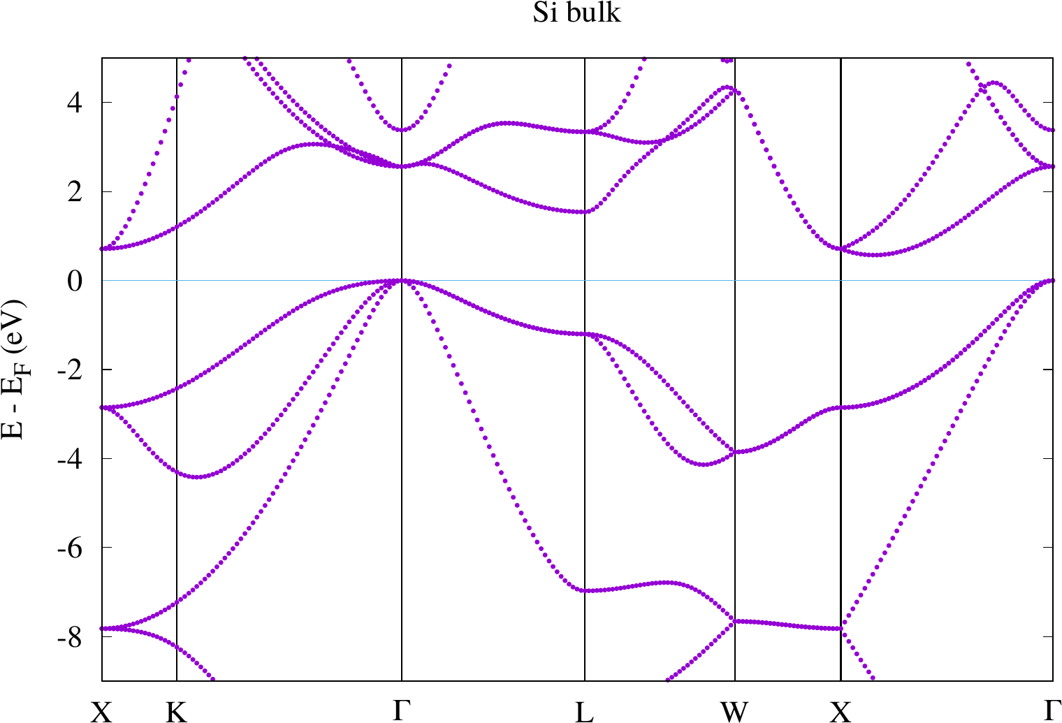
$cap=Band structure for Si with experimental lattice constant.,width=0.8\textwidth$

Where is the highest occupied state, where is the lowest unoccupied state? How large is the bandgap (grep for bandgap in the out.xml file)? Compare the result with the experimental value? How large is the difference and why is there a difference?

Beyond this quick way of plotting a band structure Fleur also writes out a file banddos.hdf. In this file the state eigenenergies are stored together with certain weights. This file can thus be used to create more sophisticated plots. The masci-tools offer a simple path to do so. The following Python script demonstrates such a usage of the masci-tools and the banddos.hdf file:

from masci_tools.io.parsers.hdf5 import HDF5Reader
from masci_tools.io.parsers.hdf5.recipes import FleurBands

from masci_tools.vis.fleur import plot_fleur_bands

filepath='banddos.hdf'

with HDF5Reader(filepath) as h5reader:
    data, attributes = h5reader.read(recipe=FleurBands)

# We are interested in each state's s-projection in the MT sphere of the 1st atom type.
weightName = "MT:1s"
# Some other weights:
# weightName = "MT:1p" # p-projection in the 1st atom type's MT sphere.
# weightName = "MT:1d" # d-projection in the 1st atom type's MT sphere.
# weightName = "MT:1f" # f-projection in the 1st atom type's MT sphere.
# weightName = "MT:2s" # s-projection in the 2nd atom type's MT sphere (if available).

# Plot the bandstructure and save to a file bandstructure.png
# If we just want a unweighted bandstrcture, we can omitt the weight argument here
plot_fleur_bands(data, attributes,
                 weight=weightName, 
                 limits={'y': (-13, 8)},
                 save_options={
                     'transparent': False,
                 },
                 show=False, #Change show to True to show the plot in a window
                 save_plots=True)

It is a slight modification of a similar script from the Fleur user guide. In this script the line

weightName = "MT:1s"

selects the $s$ character of the 1st atom type to be highlighted. Paste the script above into a text file plotBands.py in your band structure calculation directory and execute it with

python3 plotBands.py

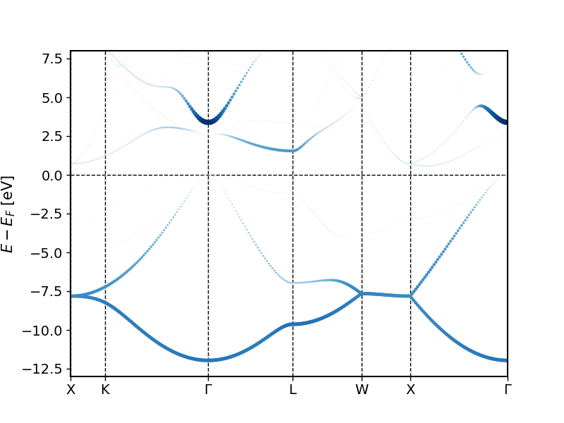
The created bandstructure.png file should look similar to the following plot.

$cap=Band structure for Si with experimental lattice constant and highlighting of the Si s character at the Si atoms.,width=0.8\textwidth$

By adapting the weightName in the script to "MT:1p" and "MT:1d" we can also highlight the p and the d character. Do this. The created band structures should look similar to the following plots.

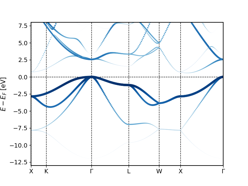
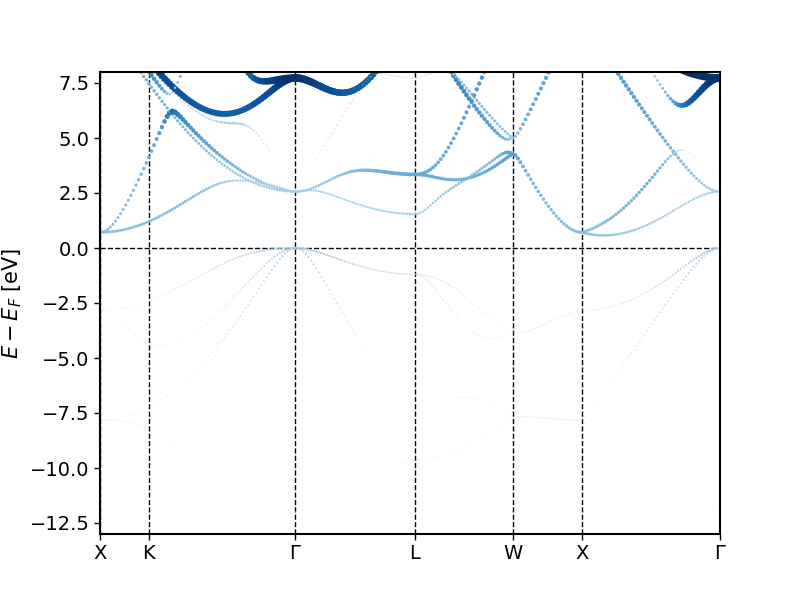
$cap=Band structure for Si with experimental lattice constant and highlighting of the Si p character at the Si atoms.,width=0.8\textwidth$

$cap=Band structure for Si with experimental lattice constant and highlighting of the Si d character at the Si atoms.,width=0.8\textwidth$

You can see in these plots that when going from lower to higher energies one first finds an $s$ -like band that hybridizes with the $p$ -like bands at higher energies. Far above the Fermi energy $E_\text{F}$ one then also observes considerable $d$ character of the bands.

1.2. Strontium band structure

Use this inp.xml file for Strontium to calculate the band structure for Strontium! Does the result look correct to you? Can it be improved? If so: How? Improve it!

Note: To change the description of a semicore state from a core electron description to a valence electron description you have to perform the following steps (also sumarized in the respective user guide section):

Identify the semicore state, i.e., the main quantum number and the angular momentum quantum number. This is best done by taking a look into the list of "coreStates" in the out.xml file of the SCF calculation (Note that every Fleur calculation moves a previously existing out.xml file in the same directory to a file out-???.xml, where the question marks indicate a number). Considering that the name of the file is out-001.xml you can extract these core state lists with grep -i state out-002.xml Semicore states feature energies that are near the valence band. Depending on the angular momentum of the state this may actually be 2 states as the fully-relativistic description for the core electrons yields a splitting of the states due to spin-orbit coupling. The list of core electron states also provides information on how many electrons there are in this state. This is the "weight".
For each atom (not atom type, group, or species) for which the description of the semicore state has to be changed add the number of related electrons to cell/bzIntegration@valenceElectrons.
Add the respective local orbital for the state (type is SCLO; n, l as identified; eDeriv 0) to the related atom species section just below the energy parameters.
Adjust the electron configuration in the atomSpecies section by moving the identified state(s) from atomSpecies/electronConfig/coreConfig to atomSpecies/electronConfig/valenceConfig (note that states in these lists are separated by spaces).

2. Exercises

2.1. Proof of orthogonality to core states

Proof $\langle u_l^c(\epsilon_c,r) \vert \dot{u}_l(E_l,r) \rangle = 0$ under the assumptions $u_l^c(\epsilon_c,r) \vert_{R_\text{MT}} = 0$ and $\frac{\partial}{\partial r} u_l^c(\epsilon_c,r) \vert_{R_\text{MT}} = 0$ . The function $u_l^c(\epsilon_c,r)$ is the wave function of a core state with eigenenergy $\epsilon_c$ . $\dot{u}_l(E_l,r)$ is the energy derivative of $u_l(E_l,r)$ and thus part of the LAPW basis.

Hint 1: $E_l$ is an energy parameter and not an eigenenergy for the Hamilton operator. $u_l(E_l,r)$ and $\dot{u}_l(E_l,r)$ are not eigenfunctions.

Hint 2: The differential equation to calculate $\dot{u}_l(E_l,r)$ is obtained by deriving $\hat{H} u_l(E_l,r) = E_l u_l(E_l,r)$ with respect to $E_l$ . The non-relativistic Hamilton operator has no energy dependence.

Hint 3: You may assume that $\langle u_l^c(\epsilon_c,r) \vert u_l(E_l,r) \rangle = 0$ has already been shown.

Results to be delivered: The proof.

2.2. Ne band structure

Note: In the following you have to modify the gnuplot script band.gnu (or the masci-tools script) such that bands up to 40 eV above the Fermi energy are displayed. The simplest way to do this is to replace in the line that starts with "plot" the last bracket by "[-10:40]" and the line before that by "set ytics -10,5,40". However the plot will not look beautiful with this single adaption.

1. Set up an input for a Ne fcc crystal with a lattice constant of $442.9~\text{pm}$ . Calculate the self-consistent solution and calculate the band structure up to energies 40 eV above the Fermi level. Note: To observe the effect to be demonstrated in this exercise it is important to not perform any parameter specifications beyond the basic unit cell setup in the inpgen input. The additional parametrization provided in the input on the example page will make the effect disappear. If you use that input remove the parametrization.

2. Copy the xml input from (1.) into a new directory and modify it in the following way: The difference to the reference calculation is supposed to be the addition of a few local orbitals constructed from the second energy derivative. Add the following line after the energyParameters xml element for the atom species:

       <lo type="SCLO" l="0" n="2" eDeriv="2"/>
       <lo type="SCLO" l="1" n="2" eDeriv="2"/>
       <lo type="SCLO" l="2" n="3" eDeriv="2"/>
       <lo type="SCLO" l="3" n="4" eDeriv="2"/>

Calculate the self-consistent solution and calculate the band structure up to energies 40 eV above the Fermi level.

3. Copy the xml input from (1.) into a new directory and modify it in the following way: The difference to the reference calculation is supposed to be the addition of a different set of local orbitals constructed from radial functions evaluated at higher energy parameters. Add the following line after the energyParameters xml element for the atom species:

       <lo type="HELO" l="0" n="3" eDeriv="0"/>
       <lo type="HELO" l="1" n="3" eDeriv="0"/>
       <lo type="HELO" l="2" n="4" eDeriv="0"/>
       <lo type="HELO" l="3" n="5" eDeriv="0"/>

Calculate the self-consistent solution and calculate the band structure up to energies 40 eV above the Fermi level.

How do the results differ? Grep for "EP" in the out.xml file. You obtain a list of the energy parameters with energies relative to the 0 of the potential. Grep for "Fermi" in the out.xml file to obtain the Fermi energy in each iteration, also relative to the 0 of the potential. How far away from the conduction band are the $s$ and $p$ energy parameters.

Results to be delivered: The three band structure plots and bandgaps.

3. Last weeks results

3.1. Cu

After performing the convergence tests we assume the following optimized parameters:

$K_\text{max} = 5.5~a_0^{-1}$
$G_\text{max} = 16.2~a_0^{-1}$
$G_\text{max}^\text{XC} = 14.5~a_0^{-1}$
$l_\text{max} = 10$
$l_\text{nonsph} = 8$
k point mesh (fcc): 26 x 26 x 26
k point mesh (hcp): 26 x 26 x 13
lower Fermi smearing energy (single shot, no optimization): 0.0001 Htr

	default parameters	refined parameters	refined parameters, low smearing	refined parameters, low smearing, c/a optimized
$a_\text{fcc} (a_0)$	$1.000764 \cdot 6.82$	$1.005883 \cdot 6.82$	$1.005896 \cdot 6.82$
bulk modulus (fcc, GPa)	$142.43$	$140.52$	$140.50$
total energy minimum per atom (fcc, Htr)	$−1655.030758$	$−1655.039326$	$−1655.039341$	$−1655.039341$
$a_\text{hcp} (a_0)$	$1.001666 \cdot 4.82247$	$1.006336 \cdot 4.82247$	$1.006345 \cdot 4.82247$	$1.006345 \cdot 4.82247$
$c_\text{hcp} (a_0)$	$1.001666 \cdot 7.87506$	$1.006336 \cdot 7.87506$	$1.006345 \cdot 7.87506$	${} \approx 1.003 * 1.006345 \cdot 7.87506$
bulk modulus (hcp, GPa)	$145.76$	$139.15$	$139.25$
total energy minimum per atom (hcp, Htr)	$−1655.0304925$	$−1655.039014$	$−1655.0390295$	${} \approx −1655.039034$
hcp-fcc energy difference per atom (meV)	$7.22$	$8.49$	$8.48$	$8.35$

Note 1: Even though the total energy difference per atom between the default parameter calculation and the one with optimized parameters is about $8.5~\text{mHtr} \approx 231~\text{meV}$ the energy difference between the hcp and fcc structure for the default parameters differs by less than $1.5~\text{meV}$ from the optimized calculation. Also the differences for the lattice constant and the bulk modulus is minimal. Lesson learned: total energy differences typically converge much faster than total energies. This implies that comparing total energies from different calculations is only meaningful if cutoff parameters and other numerical parameters are identical. Otherwise one might see the effect of these different parameters and not the total energy changes due to the intended differences in the calculation.

Note 2: On the reference computer an iteration of the default parameter calculation takes about $1~\text{s}$ . It takes about $26~\text{s}$ for the optimized parameter calculation. Considering more complex unit cells converging the total energy can be very expensive with respect to the computational demands.

Keys	Action
`?`	Open this help
`n`	Next page
`p`	Previous page
`s`	Search