
1. GW approximation
In DFT most energy eigenvalues don't have a strict physical meaning. This is different for eigenvalues obtained from the GW approximation to many-body perturbation theory. In this tutorial we will use the Spex code to perform single-shot GW calculations on top of converged DFT results to calculate band structures and other quantities. Note that there is also the possibility to perform quasiparticle self-consistent GW calculations by running fleur and Spex repeatedly after each other.
1.1. Obtaining and installing Spex
Download the Spex tarball and copy it to your preferred
spex source directory (the needed password will be provided separately). Unpack the tar with the
command tar -xf. In the now created subdirectory invoke the configure script with
MPIFC=mpiifort FCFLAGS=-I/usr/local_rwth/sw/HDF5/1.10.4/intel-intelmpi/include LDFLAGS=-L/usr/local_rwth/sw/HDF5/1.10.4/intel-intelmpi/lib ./configure --enable-mpi=yes
and compile the code with make -j4. You should now have the executables spex.inv (for systems
with inversion symmetry) and spex.noinv (without inversion symmetry) in the src subdirectory.
1.2. Si
We use our well-known Si inpgen input
Si bulk
&lattice latsys='cF', a0=1.8897269, a=5.43 /
2
14 0.125 0.125 0.125
14 -0.125 -0.125 -0.125
To generate an inp.xml file. Please use the command inpgen -f your_inpgen_input. We modify this input to let Fleur generate
the needed input for a Spex calculation. For this set the /calculationSetup/expertModes/@spex parameter to 1. Alternatively
this can also be done by adding the line
&expert spex=1 /
to the inpgen input.
Now start with converging the fleur calculation.
Also for Spex we need to set up an input file, which has to have the name 'spex.inp'. A very minimal option is:
BZ 4 4 4
KPT X=1/2*(0,1,1) K=1/8*(3,6,3)
#KPTPATH (K,1,X) 40
JOB GW IBZ:(1-10)
NBAND 80
ITERATE SR
where the lines have the following meaning:
| line | meaning |
|---|---|
| BZ 4 4 4 | Size of the kpoint mesh in the Brillouin zone. Note that this kpoint mesh is typically smaller then in DFT, as it is computationally expensive to use a fine kpoint mesh here. |
| KPT X=1/2(0,1,1) K=1/8(3,6,3) | Kpoint labels and position for extra kpoints are given. The Gamma point does not need to be specified as it is the default with the label '1'. Note that the kpoints can be given in squared bracket (cartesian coordinates) or in round brackets for internal coordinates. |
| #KPTPATH (K,1,X) 40 | This line defines the kpoint path for the band structure calculation later on. Therefore it is commented out with a '#'. It defines the path L,Gamma,X together with a step size. A larger number means a finer grid, a more detailed description can be found in the manual. |
| JOB GW IBZ:(1-10) | Defines the job Spex is supposed to do. GW refers to the GW approximation, IBZ refers to all kpoints in the Brillouin zone and (1-10) refers to the band indices for which the quasiparticle correction is evaluated. Note that you could also specify certain kpoints or bands. |
| NBAND 80 | In order to calculate the GW approximation all occupied as well as all unoccupied bands should be taken into account. Since this is impossible one needs to define a cutoff for the number of bands used. This is a parameter that needs to be converged for a precise calculation. |
| ITERATE SR | There are different options to combine Fleur and Spex. With this line Spex only takes the potential and basis set from the Fleur calculation and solves the Kohn-Sham equations itselves in a scalar-relativistic setting. |
For a complete description of the spex.inp file please consult the manual.
Now run spex.inv | tee spex.out so that the Kohn-Sham equations are solved for the k-point mesh specified in the Spex
input, followed by a single GW iteration. With the provided command the Spex output is also written to the file spex.out.
In that file you will find the output for the GW quasi particle energies per kpoint at the very end. Note that they have
a real and an imaginary part which is related to the lifetime of the respective state.
An example output for one of the k points is
#####################
### K POINT:    8 ###
#####################


--- DIAGONAL ELEMENTS [eV] ---

 Bd       vxc    sigmax    sigmac         Z        KS        HF          GW lin/dir
  1 -13.08563 -18.17892   4.60229   0.69262  -1.85030  -6.94359  -2.16392   0.30765
                          0.39695  -0.06663                      -2.16256   0.30547
  2 -13.08563 -18.17892   4.60229   0.69262  -1.85030  -6.94359  -2.16392   0.30765
                          0.39695  -0.06663                      -2.16256   0.30547
  3 -11.36082 -14.25695   2.36729   0.58404   1.95283  -0.94330   1.64201  -0.07557
                         -0.14191  -0.01382                       1.63597  -0.05178
  4 -11.36082 -14.25695   2.36729   0.58404   1.95283  -0.94330   1.64201  -0.07557
                         -0.14191  -0.01382                       1.63597  -0.05178
  5 -10.52636  -5.80617  -4.49964   0.76619  10.07850  14.79869  10.24673  -0.04298
                         -0.05193  -0.01450                      10.24642  -0.04291
  6 -10.52636  -5.80617  -4.49964   0.76619  10.07850  14.79869  10.24673  -0.04298
                         -0.05193  -0.01450                      10.24642  -0.04291
  7 -11.76633  -6.29379  -5.04721   0.74756  10.81501  16.28755  11.13182  -0.05312
                         -0.06020  -0.01907                      11.13045  -0.05319
  8 -11.76633  -6.29379  -5.04721   0.74756  10.81501  16.28755  11.13182  -0.05312
                         -0.06020  -0.01907                      11.13045  -0.05319
  9 -12.22275  -5.38366  -6.43875   0.71501  16.39871  23.23780  16.66054  -0.30761
                         -0.39566  -0.06172                      16.65944  -0.30526
 10 -12.22275  -5.38366  -6.43875   0.71501  16.39871  23.23780  16.66054  -0.30761
                         -0.39566  -0.06172                      16.65944  -0.30526
Here the real and imaginary part of the GW quasi-particle energies are listed in the last two columns. The two lines per band are
related to the linear and direct solution of the respective Dyson equation. In the column KS you can see the respective Kohn-Sham eigenenergies.
We now want to compute a band structure in order to visualize the difference between the Kohn-Sham eigenenergies (Fleur)
and the GW energies (Spex). One possible way to do so is to perform a GW calculation for each kpoint along a path in the
Brillouin zone. For this we need to find coordinates along one path. The Spex feature 'KPTPATH' helps us with this.
Uncomment the specific line in the spex.inp file and run spex once again with spex.inv -w. This generates the new file 'qpts', which
includes all the desired kpoints. Now change your spex.inp file to:
BZ 4 4 4
KPT +=(0,0,0) X=1/2*(0,1,1) K=1/8*(3,6,3)
#KPTPATH (K,1,X) 40
JOB GW +:(1-10)
NBAND 80
ITERATE SR
The kpoint after the '+=' has to be changed to one kpoint from the qpts list, followed by a Spex calculation. This has to be
performed for each k-point of the respective path, but this repeated procedure does not need to be performed manually. There is
a shell scriptspex.band prepared to do so. It can be found in the folder sh of the spex directory. Add to it the path to the
spex executable in the respective prepared line in the upper part of the script. Do not forget to uncomment this line. Now you can run it. You have
produced multiple output files from which one needs to extract the relevant values. For that there is a utility
compiled called spex.extr, which can also be found in the src directory. Please execute it
with spex.extr g -b -c spex_???.out > bandstr_gw to get the GW bandstructure and with spex.extr k -b spex_???.out > bandstr_ks
to get the DFT band structure. Inspect these files. In the first column you will find the x coordinate of the respective k point and in the
second column the related energy. In the case of the GW band structure there is also a third column containing the imaginary part of the
energies. Plot the band structures in the files with gnuplot or another plotting tool. Your plot should look similar to the following figure.
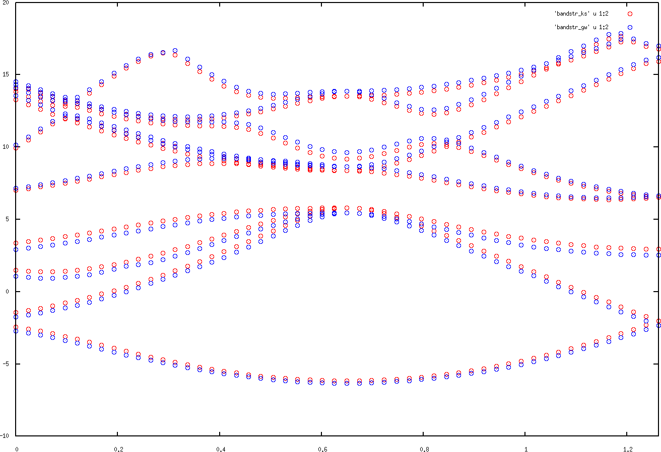
Note that the plots are shifted with respect to the Fermi energy. They also only contain the 10 bands specified in the spex.inp file. If you
want to shift the plots with respect to this you can inspect the spex.out file. In it you will find two Fermi energies. The first is related
to the Kohn-Sham system, the other one to the GW calculation. Both indicate the center of the energy gap between the occupied and unoccupied
states. Directly above the respective lines you find the energy gap. In the example calculationgrep -i -B 1 "Fermi energy:" spex.out gives:
Energy gap:       0.02619656 Ha   (  0.71284452 eV )
Fermi energy:     0.22643339 Ha   (  6.16156595 eV )
--
Energy gap:       0.04388645 Ha   (  1.19421106 eV )
Fermi energy:     0.22211361 Ha   (  6.04401875 eV )
Find out a value for the experimental band gap from the internet and compare your two results with it. Note that the GW approximation does not cover excitonic effects.
It is also possible to calculate the dielectric function. Starting with any of the two spex.inp files shown above to calculate it for the KS system you need to change the 'JOB' line
to JOB DIELEC 1:{0.0:0.2,0.0005}.
This means calculating the dielectric function from 0.0 Htr to 0.2 Htr with a step size of 0.001 Htr. This is only done for kpoint
label '1', meaning for the point with a displacement vector of (0,0,0). This is a very good assumption for optical transitions, since in this
band picture photons carry a lot of energy with only very little momentum. When you now run spex again you get the files dielec and
dielecR. The first one contains the head elements of the (bare) dielectric function and the
second one the head element of the renormalized dielectric function . The imaginary
part of the dielecR can be identified with an optical absorption spectrum (excluding excitonic effects). We will be using dielecR. Inspect this file and plot it.
An example plot for this file is shown below. Note that it was produced with an older version of Spex that used Htr units in this output. The newer Spex version uses eV.
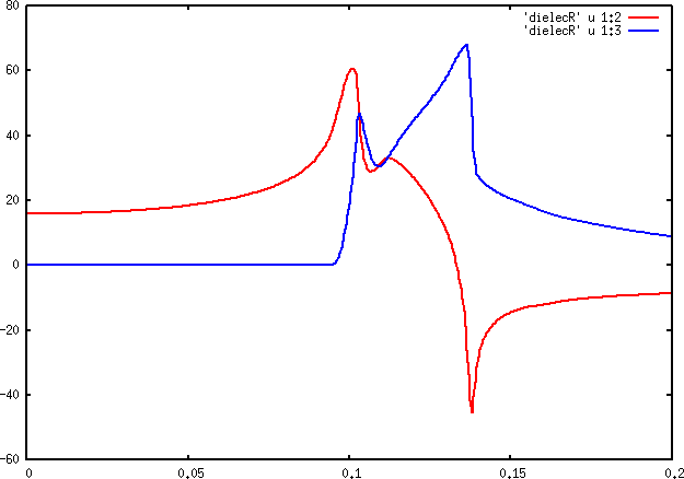
Note: To obtain an EELS spectrum from these values one would have to plot for example in 'gnuplot': 'plot "dielecR" using 1:(-imag(1/($2+{0,1}*$3))))'
Note2: Of course, it is also possible to use SPEX to calculate the dielectric function for the GW system.
Compare the gap extracted from 'dielecR' (by investigating the imaginary part) with the experimental band gap of Si. How large is the difference, why is it there?
2. Exercises
2.1. GaN
GaN crystallizes in Wurtzite (ZnS) structure. Its hexagonal unit cell ('hP' for inpgen) has the lattice parameters a=3.19 Angstrom and c=5.189 Angstrom. It features space group 186 (P63mc). The representative atoms are at (internal coordinates):
| atom species | x | y | z | Wyckoff symbol |
|---|---|---|---|---|
| Ga | 1/3 | 2/3 | 0.0 | 2b |
| N | 1/3 | 2/3 | 0.623 | 2b |
Set up the input for the material and calculate the DFT (PBE) band structure as well as the GW band structure along the path. For the GW calculation use an nband parameter of 160. Compare them. What are the band gaps in both cases? For the GW calculation also calculate the dielectric function (of the KS system) and with this the complex refractive index. According to your calculations: What wavelength does a GaN laser diode have? Look up the experimental band gap of GaN and compare your values to it.
Note 1: M = (0.0,0.5,0.0) ; K = (1/3,1/3,0.0)
Note 2: GaN does not feature inversion symmetry.
Results to be delivered: 1. Plot of the PBE band structure. 2. Plot of the GW band structure. 3. Plot of the complex dielectric function. 4. Plot of the complex refractive index. 5. Band gaps for the PBE and GW calculations.