
1. The Si lattice constant
In this tutorial the inpgen and fleur input files have to be modified. Please consult the documentation for the inpgen input and the inp.xml file for relevant aspects of these files you are not yet familiar with. You can also have a look at the inpgen example page. Note that the example inputs are far more complex than what is needed in this tutorial.
NOTE: If you base any calculation in this tutorial on input from the example page make sure to remove any explicit parameter settings in the lower part of that input. It may be that the parameters in the example inputs are chosen such that you cannot see certain phenomena this tutorial is supposed to demonstrate. Especially over the next few weeks we will investigate the dependence of calculation results on parameters. These parts of the tutorial would be affected.
1.1. Modifying inp.xml for different test lattice constants
The first predictions we want to obtain from the Fleur code are the lattice constant and the bulk modulus of Si. We already created an inp.xml file from a simple inpgen input last time. In this tutorial we will adapt this inp.xml file to perform calculations for different test lattice constants. It is important to adapt the inp.xml file and not the inpgen input since different test lattice constants in the inpgen input will cause a different parametrization in inp.xml. As a consequence the calculations would not be comparable.
The first thing we do is to adjust the maximum number of iterations we are about to perform to 40. This should be
enough for obtaining converged results for this system. The XML attribute to be adapted for this is
calculationSetup/scfLoop/@itmax.
In the FLAPW method the unit cell is partitioned into different regions. There are nonoverlapping so called
"muffin-tin" (MT) spheres centered at each atomic nucleus and an interstitial region filling the rest of the unit
cell. We want to test lattice constants in 1% steps from 97% to 103% of the lattice constant we initially provided to
inpgen. To assure that all of these calculations work we have to guarantee that for none of them the MT spheres
overlap. We already saw that inpgen yields valid input. Therefore it is enough to reduce the Si MT radius to 97%
of the already available default value. We can calculate the new radius on our own or just write the mathematical
expression into the respective XML attribute atomSpecies/species/mtSphere/@radius for the Si-1 species. The radius
has to be the same for all calculations.
Next we generate the subdirectories latt-0-97 to latt-1-03 and copy inp.xml and sym.out into each of them. In each
directory we can easily adjust a scaling factor in the respective inp.xml file to obtain the desired lattice
constant. This scaling factor is found in the XML attribute cell/bulkLattice/@scale. We perform the 7 calculations
by calling fleur in each of the subdirectories.
Check whether all calculations are converged, e.g., by looking at the direct Fleur output or by calling "grep dist
out". The total energies can be found for each iteration in the out file (grep "total energy" out) or in the out.xml
file (grep totalEnergy out.xml). We collect them in a file totalEnergies.txt with two columns: 1. scaling
factor, 2. converged total energy in Htr.
Hint: To get the last line of the grep output for the search on "total energy" (or some other term) in multiple files you might want to use (or adapt) the command
for f in $(find . -name "out"); do grep -H "total energy" $f | tail -1; done
in the parent directory.
Hint: The lines in the file should be ordered with respect to the scaling.
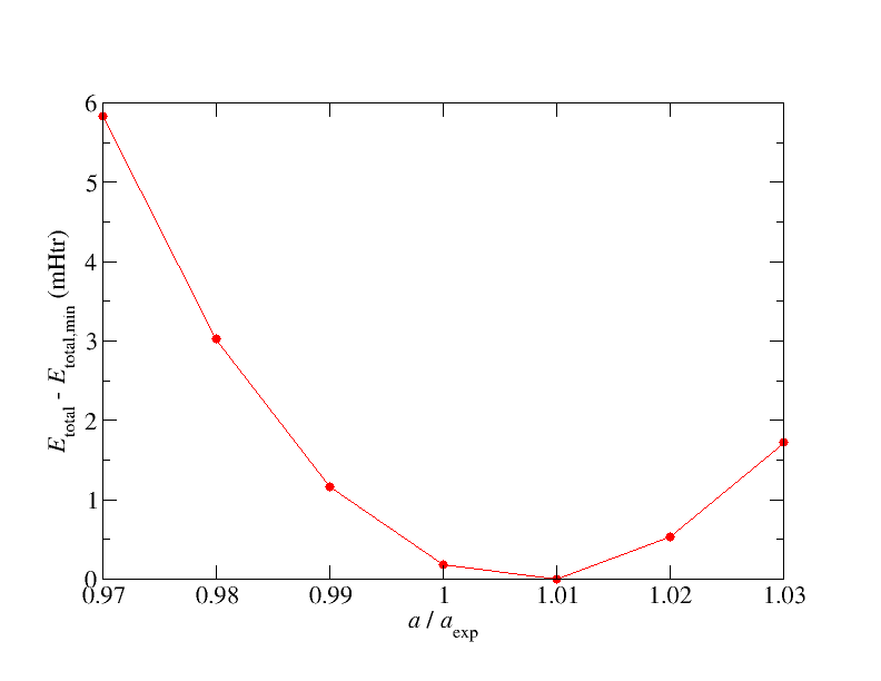
Plot totalEnergies.txt with some plotting tool like xmgrace, gnuplot, or Matplotlib. Your plot should agree with the plot below.
1.2. The Birch-Murnaghan equation of state
The calculated total energy values should be describable by the Birch-Murnaghan equation of state. As the lattice constant and the bulk modulus are parameters of this equation we fit our data to it to extract these quantities. A program that can be used to fit the data can be found here.
To use the program we copy totalEnergies.txt to totalEnergies-murn.txt and provide some more information in the first lines of the new file. An example for the additional lines is
3 # Hartree
270.107 # unit cell ratio
0.960 1.040 50 # min, max unit cell, no points
7 # no energy val
The first line sets the unit for the provided energy values (3 for Hartree). The second line is the unit cell volume for
the scaling factor 1.0. You can obtain it by calling grep volume latt-1-00/out.xml. The third line controls the output
of the program. In this example it will provide 50 energy values obtained from the fitted
equation between a scaling factor of 0.96 and 1.04. The fourth line is the number of energy values we provide as input to
the fitting program.
We store the Murnaghan fitting program in a file murn.f and compile it with a Fortran compiler like ifort by
invoking ifort -o murn.x murn.f.
We execute the program with ./murn.x < totalEnergies-murn.txt.
The program writes out the equilibrium lattice constant (alat) in terms of the optimal scaling factor. Convert it to Angstrom or a_0. The bulk modulus (b0) is written out in MBar. Convert that to GPa. Finally compare the obtained values to experimental values availaible at wikipedia, WebElements, or other freely available sources (normally we would compare to experimental or theoretical results from scientific papers). Plot the energy values obtained through the fitting procedure together with those obtained from the DFT calculation. The result should agree with the following plot:
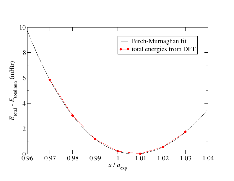
By visually inspecting the plot it is obvious that the Birch-Murnaghan fit is in excellent agreement with the total energies calculated with DFT. It should be like that. Whenever you try to make such a fit and the agreement is considerably worse, there is a problem in your calculations.
1.3. The lattice constant with LDA
In principle, density functional theory is exact. However, for one of the energy terms involved in the description there is no exact expression for its dependence on the charge density known. This is the eXchange-Correlation (XC) energy, for which approximations are used. A simple approximation for this term is the Local Density Approximation (LDA), a slightly more sophisticated approach are Generalized Gradient Approximations (GGAs) and there are also many formulations of the XC energy that go beyond these approximations. Both LDA and GGAs are used in numerous parametrizations, typically named by an acronym, e.g., PBE or VWN.
By default inpgen sets up the inp.xml file such that the PBE GGA XC functional is used. We want to compare the results we
obtained with this functional with analogous LDA calculations. For this we change the calculationSetup/xcFunctional/@name XML attribute in
the inp.xml file to "vwn" and perform the steps described above in a new directory again for this Vosko-Wilk-Nusair
parametrization of the LDA XC functional.
Compare the lattice constant obtained from the PBE calculations with the one from the VWN calculation. Which one is larger? Note that the observed overbinding and underbinding is a rather typical trend between LDA and GGAs.
2. Exercise: Some more lattice constants
Note: The results of the exercises have to be handed in before Wednesday next week either by direct message in the Slack channel or by email. The students are encouraged to discuss and help each other (via Slack) in getting the calculations to run (unit cell setup, sharing useful scripts, and so on). But they are also supposed to do the calculations and extract the results by themselves.
For many materials lattice constants predicted by DFT calculations with local or semilocal XC functionals match the experimental values with a typical deviation of only a few percent. The bulk modulus typically deviates by 10-20%. Thus, many DFT structure predictions are very good. In the excercises we want to test some limiting cases. For each example make sure that you calculate at least 2 test lattice constants on each side of the total energy minimum.
2.1. fcc vs. hcp Cu
The fcc lattice features an ABCABC stacking of the close-packed atomic monolayers. The hcp lattice is very similar to this but features an ABABAB stacking. This similarity yields tiny energy differences between the respective structures. We compare these structures for Cu which features an fcc ground-state structure with a lattice constant of 3.61 Angstrom. Calculate the PBE equilibrium nearest-neighbor distance for the atoms in fcc and hcp Cu by performing calculations with different test lattice constants. For hcp Cu we assume the optimal c/a ratio for the packing of spheres. Plot the "energy per atom" vs. "nearest neighbor distance" values for both calculations in one plot. According to your plot: Which is the ground-state structure? How large is the energetic difference per atom in meV?
Note 1: You may want to use an example input for another element as starting point for the hcp calculations. Cobalt has an hcp ground-state structure. Make sure that you adapt every relevant parameter and get rid of additional unwanted parameter specifications in the example input. Also be aware that there are different ways of defining an hcp unit cell. The input generator also generates a file struct.xsf. This is an XCrysDen structure file. You can open it with the free programs XCrysDen or Vesta to visualize the generated unit cell and check whether it agrees with your assumptions. It is also a good check to compare the generated parameters for the atom species with the fcc setup. If the differences are very large there is probably a problem in the inpgen input.
Note 2: The choice of the kPoint set for the Brillouin zone integration is an important aspect to obtain comparable results. To obtain comparable kPoint sets we add to the end of the inpgen input for the fcc calculation
&kpt div1=14 div2=14 div3=14 /
and to the one for the hcp calculation
&kpt div1=14 div2=14 div3=7 /
Note 3: To assure that the calculations are comparable we also have to set some numerical parameters to the same values. These are provided in the XML attributes:
calculationSetup/cutoffs@Kmax
calculationSetup/cutoffs@Gmax
calculationSetup/cutoffs@GmaxXC
atomSpecies/species/mtSphere@radius
atomSpecies/species/mtSphere@gridPoints
atomSpecies/species/mtSphere@logIncrement
atomSpecies/species/atomicCutoffs@lmax
atomSpecies/species/atomicCutoffs@lnonsphr
Choose one of the inp.xml files as reference for the values and set the attributes in the other inp.xml file to the same values.
Results to be delivered: Single plot with "total energy per atom" vs. "nearest-neighbor atom distance" together with Birch-Murnaghan fits for both, fcc and hcp; Calculated energy difference per atom between optimized fcc and hcp structures in meV; Optimzed nearest-neighbor atom distances; Bulk modulus for both structures.
2.2. fcc Ar
An Argon noble gas crystal in fcc structure has an experimental lattice constant of 5.26 Angstrom. Which equilibrium lattice constant do you obtain with the PBE functional?
Note 1: This system is bound by Van-der-Waals interactions which are not well-described by conventional local or semilocal exchange-correlation functionals. We therefore expect very bad results. This exercise is meant to make the students aware of the importance to understand the dominant interactions in a material to perform reasonable calculations.
Note 2: Be patient in searching the total energy minimum. This system is bound, even with the PBE functional.
Results to be delivered: Plot with calculated total energies for different test lattice constants together with a Birch-Murnaghan fit; Calculated equilibrium lattice constant; Relative deviation of calculated equilibrium lattice constant from experimental value.