
1. Noncollinear magnetism and force theorem
For many materials the magnetic unit cell is neither ferromagnetic nor antiferromagnetic but features a more complex magnetic structure in which the orientation of the magnetic moments related to the different atoms changes within the unit cell. Such magnetic structures are called noncollinear and may be caused by different circumstances. One possible cause is magnetic frustration, i.e., a preferred alignment of the magnetic moments at the different atoms is in contradiction with the geometry of the system. Another cause may be spin-orbit coupling. In this tutorial we will calculate several noncollinear magnetic structures for a magnetically frustrated system.
In Fleur noncollinearity is treated such that within the MT sphere of a certain atom a single magnetization direction is assumed in the setup of the Hamiltonian but this direction can differ between the atoms. The magnetization directions in the MT spheres are given in terms of the two angles and analogous to the and angles used for the specification of the SQA in SOC calculations. In the interstitial region between the MT spheres the orientation of the magnetization continuously changes.
1.1. Noncollinear magnetism in a Cr Monolayer with hexagonal lattice geometry
NOTE: While performing the calculations for this example you should download the visualization tool XCrysDen and get it to run if it doesn't already run on your computer. You will need it. Alternatively you can also work with VESTA.
NOTE 2: This tutorial example is motivated by the article Ph Kurz, G. Bihlmayer, and S. Blügel, Noncollinear magnetism of Cr and Mn monolayers on Cu(111), Journal of Applied Physics 87, 6101 (2000).
For Cr atoms the preferred magnetic ordering is antiferromagnetic. In a triangular lattice this is not possible and such a setup therefore is an example for a prototypical magnetically frustrated system. To obtain such a lattice for Cr one can grow a single layer of Cr atoms on a Cu(111) surface. In such a sample the Cr atoms will occupy the positions of Cu atoms in the respective layer. As an approximation to such a setup we calculate an unsupported Cr monolayer with atoms at such positions. Assume an fcc Cu crystal with a lattice constant of . This translates into a nearest-neighbor distance between the atoms of . In this tutorial example we consider a unit cell of two atoms, and in the exercises a unit cell containing three atoms is investigated. The setup for this example is sketched in the following figure.
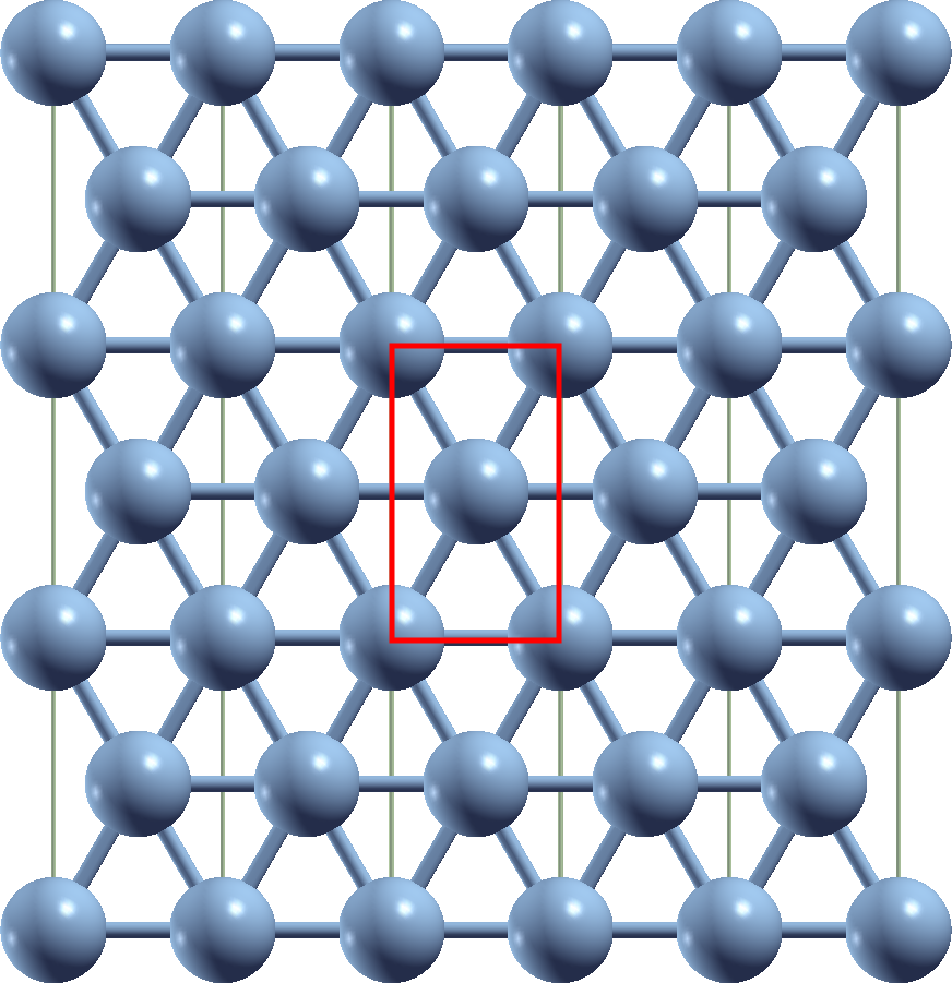
Calculate the lattice parameters for the sketched unit cell and set up an inpgen input for such a film system with two inequivalent Cr atoms.
Calculations with noncollinear magnetism require parameters that are not provided within the default Fleur input template
generated by the input generator. We have to use inpgen with the -noco command line option to obtain a template containing
such parameters. Generate a Fleur input file in this way.
To actually perform the calculations we also have to make some adjustments to the Fleur input file:
-
Set the number of iterations to 90: This system does not show trivial convergance behavior. Note that the 90 iterations might not be enough for some of the calculations. For such a case run Fleur multiple times and remove the file "mixing_history" between the runs.
-
Set
/calculationSetup/scfLoop/@maxIterBroydto 10. This forces the deletion of the charge density mixing history after every 10 iterations of the SCF loop. This is a measure to obtain a more benign convergence behavior. -
Set
/calculationSetup/coreElectrons/@ctailto "F". Noncollinear features are incompatibel with this feature. The switch turns on a certain treatment of the part of the core electron density that reaches out of the MT spheres. -
Set
/calculationSetup/magnetism/@l_nocoto "T". This actually switches on the noncollinear calculation mode. -
Set
/calculationSetup/magnetism/mtNocoParams/@l_mperpto "T". This activates the calculation of the offdiagonal (Spin-Up - Spin-Down) part of the density in the MT spheres. We only need this for visualization purposes. -
Reduce all MT radii to 90% and to keep the product of the MT radii and constant increase accordingly.
-
Change the XC functional to the LSDA formulation of Moruzzi, Janak, and Williams (choose "mjw" for
calculationSetup/xcFunctional/@name). This is just done in accordance with the article cited above. -
Increase the initial magnetic moments to . This is done because lower initial magnetic moments may lead to the calculation of a nonmagnetic self-consistent solution. All magnetic moments are supposed to be positive. An example for setting the magnetic moments accordingly by modifying the occupations for the initial electron configuration is
         <electronConfig flipSpins="F">
            <coreConfig>(1s1/2) (2s1/2) (2p1/2) (2p3/2)</coreConfig>
            <valenceConfig>(3s1/2) (3p1/2) (3p3/2) (4s1/2) (3d3/2) (3d5/2)</valenceConfig>
            <stateOccupation state="(4s1/2)" spinUp=".50000000" spinDown=".50000000"/>
            <stateOccupation state="(3d3/2)" spinUp="8.0/5.0" spinDown="2.0/5.0"/>
            <stateOccupation state="(3d5/2)" spinUp="12.0/5.0" spinDown="3.0/5.0"/>
         </electronConfig>
We will perform calculations with different in-plane magnetic setups. To restrict the SQA to the plane of the film set
/atomGroups/atomGroup/nocoParams/@beta to "Pi/2.0" for both atoms.
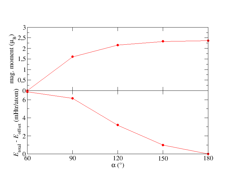
For one of the atoms keep the angle (/atomGroups/atomGroup/nocoParams/@alpha) constant at but vary it for the
other one in steps of "Pi/6.0" from "2.0*Pi/6.0" (this is the hardest calculation that took about 430 iterations in the test run)
to "Pi" in different subdirectories. Calculate the self-consistent solutions for each of these setups.
Plot the total energy and the magnetic moment in dependence of . Your results should be similar to the following plot.
The following second part of the exercise is cancelled because there is a related bug in the current release version!
We now want to visualize for the case the spatially-dependent orientation of the magnetization within the
unit cell. For this copy everything from this calculation to a new directory and in this directory change in the inp.xml
file /output/plotting/@iplot to "1" and /output/plotting/@polar to "T".
We also want to adapt the region and the resolution in which the visualization takes place. For this we change
the contents of the output/plotting/plot tag. In the test calculation this is modified to
<plot TwoD="T" grid="35 60 35" vec1=" 1.0 0.0 0.0" vec2=" 0.0 1.0 0.0" vec3=" 0.0 0.0 1.0" zero=" -0.25 -0.25 0.0" file="plot"/>
In comparison to the default this add the entry grid="35 60 35" which specifies the number of voxels in the generated
volumetric data file in the directions of the 3 vectors defined in same xml element. Make sure that the entry 60 coincides
with the elongated dimension of your unit cell. We also change the offset for the generation of the plot this is done in
the zero=" -0.25 -0.25 0.0" entry.
Invoke Fleur for this input. Now several XCrySDen structure files for the visualization of different quantities are generated. For a description of each of these outputs consult the respective page in the user guide.
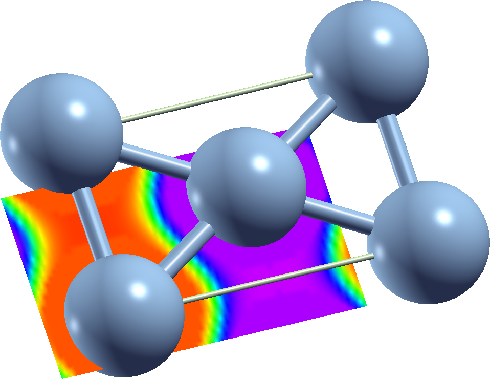
We are interested in the denOutWithCore_Aphi.xsf which encodes the direction of the inp-plane magnetization of the film by providing the
angle at every point in the unit cell for the provided input density.
Run XCrysden and open this file. Go to Tools->Data grid and press "OK". You can then define different parametrizations for the visualization. Play with it, use a rainbow color coding together with a linear scale. If you open one of the other files not related to angles you will realize that most of the density and magnetization density is found very near to the atom positions.
For the magnetization directions you should be able to obtain a color-encoded visualization similar to the following figure.
If you have time you can also go to earlier tutorial examples from which you have self-consistent solutions and generate charge density plots for those. For example Si should have a large density between the atoms due to the covalent bonding. Is this really the case?
2. Exercises
2.1 Three-atom unit cell of the Cr film
Extracting parameters for a Heisenberg model from DFT calculations with simple magnetic configurations of a Cr film and performing simulations on the basis of this model predicts that the ground state for this system features an in-plane rotation of 120° between the magnetic moments of neighboring Cr atoms. It turns out that DFT calculations for such a magnetic configuration and similar configurations agree with this prediction. Note that such an agreement between Heisenberg model predictions and more accurate DFT calculations is not for all systems the case.
Here we want to perform the DFT calculation for the magnetic ground-state structure.
Print out or draw a reasonable region of a triangular lattice (you can use the sketch above) and select a triangle of neighboring atoms. For this triangle draw arrows at the atoms pointing from the center of the triangle outwards. Assume that these arrows indicate the magnetic moments. Draw the magnetic moments for the other atoms according to the 120° rotations from atom to atom.
On the basis of this drawing select a magnetic unit cell containing three inequivalent atoms. Verify that the repetitions of this unit cell feature the same magnetization. Set up an inpgen input with this Cr film unit cell and the nearest-neighbor distance provided in task 1.1. Generate a Fleur input with parametrization for noncollinear setups and adapt the parameters as good as possible to the Fleur input files from task 1.1. Set the SQAs at the different atoms according to the construction of the magnetic unit cell.
Perform a Fleur calculation to obtain the ground-state density for this setup. Compare the total energy per atom to the energetically most likely configuration from task 1.1. Plot the magnetization direction at each point in the unit cell in the film plane.
Results to be delivered: 1. The comparison of the total energy per atom to task The following is cancelled: 1.1. 2. A plot of the magnetization directions at every point in the unit cell in the film plane.
2.2. Magnetocrystalline anisotropy in Co revisited with the magnetic force theorem
Last week the magnetocrystalline anisotropy in Co was determined by performing self-consistent calculations for different spin-quantization axes (SQAs). There is also a faster way to do this. According to the magnetic force theorem already single-shot calculations for different SQAs (only determination of the eigenvalue sum for a fixed input density) on top of a representative self-consistent density for one SQA should provide reasonable approximate results. To do this we have to add a special XML element to one of the inp.xml files for Co from last week. Choose the one with and and add
   <forceTheorem>
      <MAE theta="0.0 0.5*Pi 0.25*Pi 0.5*Pi" phi="0.0 0.0 0.0 0.5*Pi" />
   </forceTheorem>
directly after the output section of the inp.xml file. In the forceTheorem XML element we provide the parametrization for such
a calculation. It can be used to determine the magnetocrystalline anisotropy energy (MAE), for other quantities like the
parameters of the Dzyaloshinskii-Moriya interaction (DMI),
or for the determination of spin-spiral dispersion relations.
For the MAE calculation a MAE xml element has to be provided that features the two xml attributes theta and phi, both representing a list of respective angles. The i-th angles from both lists define the i-th SQA. The example above provides exactly those angles that were also used last week.
Run fleur with this input to first calculate a self-consistent density. The force theorem calculation starts if the iteration number of the current run equals the maximum iteration number specified in the inp.xml file or the convergence criterion is reached. Note that the usage of the force theorem replaces the 4 self-consistency calculations from last week by a single self-consistency calculation. We thus nearly obtain a factor 4 speedup.
In the out.xml file you should now have a "Forcetheorem_MAE" section in which a list with the different angles together with respective eigenvalue sums is provided. Determine the "K_i" parameters from last weeks uniaxial MAE model and compare them to the parameters determined with self-consistent calculations.
Results to be delivered: The eigenvalue sums for each combination of angles and the parameters and for the MAE model obtained from these eigenvalue sums.