
Spin spiral calculations
Objectives
- Understanding the use of the spin-spiral mode of FLEUR.
- Setting up a spin-spiral setup using
inpgen. - Running for different q-vectors.
Introduction
Often the magnetic ground state in a material is neither ferromagnetic nor antiferromagnetic but a noncollinear magnetic structure. In this example we will investigate a special case of such a noncollinear magnetic structure in fcc Fe: A spin spiral in z-direction, where the magnetization rotates in the xy plane.
In its ground state Fe crystallizes in a bcc structure, but it is also possible to synthesize Fe in an fcc structure, e.g., fcc Fe clusters may form by fast annealing of Fe in a Cu matrix. As this is a small and simple unit-cell we use it here to demonstrate the spin-spiral feature.
```{note} FM/AFM as special cases It is obvious that the FM and AFM configurations are special cases of such spin spirals. In the FM case the rotation vanishes and in the AFM case the rotation from one atomic layer to the next is . The exception here is that in Fleur a spin-spiral calculation assumes, according to the provided angles, a collinear orientation of the magnetization within the MT spheres, while in the interstitial region the magnetization is allowed to vary its direction in space. Hence a spin-spiral calculation of these collinear configurations in principle allows more a noncollinear behavior of the magnetization in the interstitial region.
FLEUR can efficiently describe such spin spirals by employing the generalized Bloch theorem. It allows us to describe the FM and AFM configurations, as well as all other magnetic configurations covered by such a spin spiral in a unit cell with a single Fe atom.

In the ```FeSpinSpiral``` directory the ```inpFeSpinSpiral.txt``` is a starting point for such a calculation. Change into that directory and display the file.


```bash
cd FeSpinSpiral/ ; cat inpFeSpinSpiral.txt
It describes a primitive fcc unit cell. The &qss entry is the spin-spiral vector q associated with the general expression for the magnetization in the MT spheres
where is the lattice vector pointing from the origin to unit cell , is the position of atom in the unit cell, is the cone angle between the magnetic moment of atom and the rotation axis, and is an atom-dependent phase shift.
Multiplying the q vector specified in the inpgen input with the reciprocal Bravais matrix of the investiated system shows that it actually describes a spin spiral in z direction. With the expression for the magnetization then descibes the FM configuration for and the AFM configuration for .
```{note} Usage hints for inpgen and spin-spirals
- Spin spirals break the symmetry of the chemical unit cell. Hence, specifying the
q-vectorforinpgenensures that the correct symmetry is used. - Setting the spin-spiral vector indicates that a non-collinear setup is required. So this would usually already be enough to generate the switches in
inp.xmlused in non-collinear setups. However, - Spin spirals in FLEUR rotate around the
z-axis. Hence must be different from zero to have an actual spin spiral. Here, we use the vector of the magnetization at the atom to rotate the magnetization to an angle of
Generate the Fleur input file.


```bash
inpgen -f inpFeSpinSpiral.txt
```{warning} Reduce computational effort As we have broken the symmetry, we have very many k-points. For the purpose of this tutorial, before starting the spin-spiral calculation, we should reduce the computational demands by using a reduced k-point mesh with points.
We generate it by invoking


```bash
inpgen -inp.xml -kpt grid=8,8,8
Now we want to prepare the inp.xml file to perform a series of setups with different q-vectors. To simplify this process we will use the possibility to define variables in inp.xml. We will replace the q-vector definition to
<qss>q q .0000000000</qss>
and define the variable q by adding to the top of the inp.xml after the comment
<constants>
<constant name="q" value="0.0"/>
</constants>
``{warning} Please modify inp.xml by
1. Set/calculationSetup/scfLoop/@itmaxto"50".
2. Select the new k-point mesh by setting/cell/bzIntegration/kPointListSelection/@listNameto"default-3".
3. Modify theqsstag as decribed above.
4. Add theconstants` section.
We will calculate spin spirals of the form $(q, q, 0.0)$ for q from 0.0 to 0.5 in steps of 0.125. For this create directories ```qXY-0.0``` to ```qXY-0.5```. Copy all xml files needed for these calculations to each of the directories.


```bash
for q in 0.0 0.125 0.250 0.375 0.5
do
    mkdir qXY-$q
    cp *.xml qXY-$q
done
Now we have the same input in all directories. To run for different inputs we can use the feature of FLEUR allowing to modify the input using a command line switch. So we again loop over all configurations
for q in 0.0 0.125 0.250 0.375 0.5
do
    cd qXY-$q
    fleur_MPI -xmlXPath "/fleurInput/constants/constant[1]/@value=$q" #here we modify the first constant (the q)
    cd -
done
```{warning} Long runtime! Unfortunately, this will now take quite some time to run. But once we are done we can look at the results.
Extract the total energy for the self-consistent solution of each calculation, e.g, by invoking


```bash
for q in 0.0 0.125 0.250 0.375 0.5
do
    echo $q `grep "total energy" qXY-$q/out |tail -1|cut -d= -f 2`
done
We now want to plot the spin-spiral dispersion. For this we store the relevant data in a two-column text file and use a prepared Python script to plot the stored data.
``{warning} Create spin-spiral data file
Create a text file 'spinSpiral.txt' that has two columns. Put the
q` value of each calculation in the first column and the respective total energy (in Htr) in the second column.
The script we use for the plotting is provided in the file 'plotSpinSpiral.py' of the main directory of this tutorial section. Inspect it.


```bash
cat ../plotSpinSpiral.py
We run the script to create the plot. You are, of course, free to adapt and use the script for all your needs, even beyond this tutorial.
python ../plotSpinSpiral.py
The script will generate a file 'spinSpiral.png' that you can display by clicking on it in the file browser on the left. Your result should look similar to every 2nd point from the following plot.
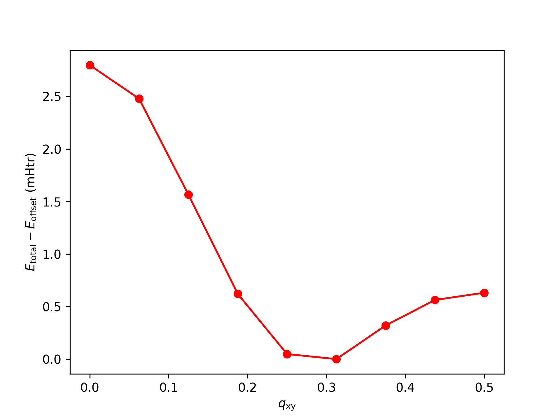
We can see that there is a minimum for a q value that is neither in the center nor at the boundary of the Brillouin zone.
The aiida workflow
Instead of the "shell magic" we performed above, one can of course also use a workflow provided by the AiiDA-FLEUR plugin. This workflow is called ssdisp_conv as it calculates the dispersion of a spin-spiral using fully converged solutions.
aiida-fleur launch ssdisp_conv
Here you are now informed that starting the workflow is slightly more complex than in the examples before. The inp.xml you provide is of course not sufficient to determine which q-vectors to calculate and hence the specification of the workflow parameters is required. We first create a template again:
aiida-fleur launch ssdisp_conv -wf template.json
cat wf_ssdisp_conv.json
As you might have expected, there are basically two parameters to specify:
1. The beta angle to use. You can provide here different angles for different atoms (given by their labels) or a single angle for all atoms as shown in the template.
2. The q-vectors to use. For clearer reference, these are provided with a label.
```{warning} Modify the file You might now want to adjust the file to provide the same q-vectors as above or others you want to calculate.
```bash
aiida-fleur launch ssdisp_conv -wf  wf_ssdisp_conv.json
As usual for the command line interface, the results of the workflow are provided in a json file:
cat ssdisp_conv.json
Learn more:
In FLEUR the spin spiral is always rotating around the z-axis. By choosing the Euler angle in this tutorial we created a "flat" spiral. You can also change this angle to a smaller angle to have a "coned" spiral. But be careful, by setting you end up having no spiral. So you could extend this example by looking at different cone angles of the spin-spiral.
More info on spin-spirals and the workflow discussed here is also found here: * https://www.flapw.de/MaX-7.0/documentation/spinSpirals/ * https://aiida-fleur.readthedocs.io/en/latest/user_guide/workflows/ssdisp_conv_wc.html