
Spin-orbit coupling
In this tutorial we will perform calculations related to physics in which spin-orbit coupling (SOC) plays an important role. In calculations without explicit treatment of noncollinear magnetism Fleur treats SOC in so-called second variation. This means that a conventional Hamiltonian matrix, i.e., a Hamiltonian matrix with a scalar-relativistic description in the MT spheres, is set up and diagonalized. After diagonalization the eigenfunctions are used as a new basis for which a new Hamiltonian matrix with SOC is set up and diagonalized again to obtain the final energy eigenvalues and eigenfunctions.
This calculation procedure implies that the number of eigenfunctions calculated in the first step now
becomes a cutoff parameter defining the basis set size for the second step. This parameter can be set in
/calculationSetup/cutoffs/@numbands. A value of zero indicates that a material-dependent default value is chosen
by the program. In principle SOC calculations have to be converged with respect to the numbands parameter. Due to time
limitations in this tutorial we will not do this but you are free to perform convergence tests to get a feeling for the relevance of
this parameter. Since some of the investigated quantities are sensitive to very small energy differences a significant
quantitative dependence on the cutoff parameters is expected.
Magnetocrystalline anisotropy of hcp Co
In perfect infinite ferromagnetic crystals the preferred magnetization direction is determined by spin-orbit coupling. In this example we will calculate the energy difference between different magnetization directions. Note that this typically is a very small quantity. Also be aware that magnetocrystalline anisotropy is not the only source of magnetic anisotropy. For example, in finite systems the shape of the sample also contributes to the magnetic anisotropy.
As example system we choose hcp Co. An inpgen input inpCo.txt is available in the Co subdirectory. Change into that directory and inspect the file.
export THOME=$PWD #Save tutorial home-dir
cd Co ; cat inpCo.txt
Note the line "&soc 0.10 0.37 /". With this line we define a spin quantization axis (SQA) in terms of the two angles and (spherical coordinate system). These are not the angles we will use in the actual calculations. We choose these angles in the inpgen input because the SQA breaks the symmetry of the crystal. Here we want to have the freedom to choose any other SQA after generating the inp.xml file. So we need to define an axis that breaks as many symmetries as possible. Otherwise a later choice of another axis in the inp.xml file may be incompatible to the here detected symmetry operations.
The line "&kpt div1=9 div2=9 div3=5 /" defines a k-point mesh directly in the inpgen input. As no name is provided for this mesh and it is the only k-point mesh specified in this file it overrides the default.
Generate the Fleur input.
inpgen -f inpCo.txt
In the inp.xml file the angles appear in /calculationSetup/soc/@theta and /calculationSetup/soc/@phi. The SOC
calculation is activated with the XML attribute calculationSetup/soc/@l_soc. If there is a spin quantization axis
defined in the inpgen input spin-orbit coupling is activated by default.
We will need a few more iterations than are performed by default.
Modify the inp.xml file by setting /calculationSetup/scfLoop/@itmax to "25".
To investigate different SQAs prepare separate directories for each SQA and copy all xml files to each of these directories.
- theta="0.0", phi="0.0" (z axis)
- theta="Pi/4.0", phi="0.0"
- theta="Pi/2.0", phi="0.0" (x axis)
- theta="Pi/2.0", phi="Pi/2.0" (y axis)
mkdir th-0.00-ph-0.00 ; mkdir th-0.25-ph-0.00 ; mkdir th-0.50-ph-0.00 ; mkdir th-0.50-ph-0.50
cp *.xml th-0.00-ph-0.00/ ; cp *.xml th-0.25-ph-0.00/ ; cp *.xml th-0.50-ph-0.00/ ; cp *.xml th-0.50-ph-0.50/
Adapt in each of the directories the inp.xml file to the respective SQA, e.g., in the th-0.50-ph-0.50 directory set
<soc l_soc="T" theta="0.50*Pi" phi="0.50*Pi" spav="F"/>
Perform the Fleur calculation in each directory.
cd th-0.00-ph-0.00/ ; fleur_MPI ; cd -
cd th-0.25-ph-0.00/ ; fleur_MPI ; cd -
cd th-0.50-ph-0.00/ ; fleur_MPI ; cd -
cd th-0.50-ph-0.50/ ; fleur_MPI ; cd -
Extract the converged total energy for each of the calculations. hcp Co is an uniaxial system, i.e., the magnetocrystalline anisotropy in the x-y plane is negligible. Verify that the total energy difference between calculations 3 and 4 is much smaller than the difference to calculation 1. What is the "easy axis" (energetically most preferable), what is the "hard axis"?
for f in $(find . -name "out"); do grep -H "total energy" $f | tail -1; done
Depending on the unit cell there are different models to describe the magnetocrystalline anisotropy. For uniaxial systems the total energy in dependence of the magnetization direction is expressed by the equation
In approximation we assume this expansion in terms of powers of sines of to end after the term. Use the total
energies from calculations 1, 2, and 3 to set up a system of linear equations and determine the coefficients ,
, and . In the calcCoefficients.ipynb you will find a Python script that you can modify to do this.
What are the values of the coefficients you calculated?
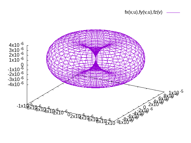
We want to visualize the anisotropy. For this we ignore the term. Plot it. For this adapt the gnuplot script in the file plotEnergySurface.plt by plugging in and . It will generate a file energySurface.png with the visualization.
cd $THOME ; gnuplot < plotEnergySurface.plt
The result of plotting the magnetic anisotropy is a file surface.png that should be similar to the plot below (not identical due to slightly different parameters). The distance between the origin and a point on the surface is the energy advantage the easy axis has over the axis in the direction of the point on the surface.
Note that the procedure of determining (extended) Heisenberg model parameters is similar to what is sketched in this example for the magnetocrystalline anisotropy: One performs DFT calculations for different magnetic configurations and plugs the results of these calculations in equation systems where each equation relates to the respective configuration in the Heisenberg model.
Force theorem for the magnetocrystalline anisotropy
Calculating many different magnetic configurations self-consistently may be very time consuming. To get an approximate result for the differences between the investigated magnetic configurations one can also obtain the self-consistent solution just for one of the configurations and then modify the magnetic configuration on top of this self-consistent solution but perform only a single iteration to calculate the eigenvalues and eigenstates. As an approximation the differences in the total energies of the converged calculations can then also be obtained as the difference in the eigenvalue sums for the different configurations. This is the magnetic Force theorem.
In this example we will test this for the the magnetocrystalline anisotropy calculated above.
Collect from your , calculation all three input xml files and store them in a new directory.
cd $THOME/Co ; mkdir ForceTheorem ; cd th-0.00-ph-0.00 ; cp *.xml $THOME/Co/ForceTheorem/ ; cd $THOME/Co/ForceTheorem/
Modify in that directory the inp.xml file by adding the following section directly below the /output section:
   <forceTheorem>
      <MAE theta="0.0 0.25*Pi 0.5*Pi 0.5*Pi" phi="0.0 0.0 0.0 0.5*Pi" />
   </forceTheorem>
The presence of this section indicates to Fleur that after reaching self-consistency the respective Force theorem step has to be performed. In this case we specify the usage of the force theorem for the calculation of the magnetocrystalline anisotropy energy (MAE). The lists of angles specified in the respective MAE tag are the same as those we used before. For the i-th configuration the i-th entries of the lists are used.
Perform the fleur calculation.
cd $THOME/Co/ForceTheorem/ ; fleur_MPI
The Force theorem results for the different configurations can be obtained from the out.xml file. A good way of obtaining them is via the command grep ev\-sum out.xml. ev-sum denotes the eigenvalue sum for the respective calculation. Use the Python script from above to obtain the coefficients and also from the eigenvalue sums and visualize the result. How large is the deviation from the original determination of these coefficients? Keep in mind that this calculation was about 4 times faster since we only obtained a self-consistent result for one of the configurations.
grep ev\-sum out.xml
Rashba effect in BiTeCl
The Rashba effect, similarly to the Dresselhaus effect, is a band splitting due to spin-orbit coupling that appears in systems with broken inversion symmetry. While the Rashba effect appears in low dimensional systems (films, heterostructures) and uniaxial bulk systems, the Dresselhaus effect is observed in cubic bulk systems. In this exercise we calculate the Rashba splitting in bulk BiTeCl. Note that it also appears in other bismuth tellurohalides (BiTeX with X=Cl,Br,I).
BiTeCl features a hexagonal unit cell (use latsys='hP' for inpgen) with 6 atoms and the lattice parameters
Angstrom and Angstrom. The inpBiTeCl.txt inpgen input in the BiTeCl directory represents such a unit cell.
Change into that directory and inspect the file.
cd $THOME/BiTeCl ; cat inpBiTeCl.txt
We will calculate this system without spin polarization. In such a case the choice of the SQA is not important, but some SQA should be specified in the inpgen input. We choose one that does not break too many symmetries. Also note that we specified two different k-point sets in the inpgen input. Both feature relatively few points to reduce the computational demands. The second k-point set is a user-defined k-point path that deviates from the default path for this unit cell.
Generate the Fleur input.
inpgen -f inpBiTeCl.txt
Increase in inp.xml the /calculationSetup/scfLoop/@itmax parameter to "30". We again need some more iterations.
Create the directories withSOC and withoutSOC and copy all xml files to these directories.
mkdir withoutSOC ; mkdir withSOC
cp *.xml withoutSOC/ ; cp *.xml withSOC
In the withoutSOC directory set /calculationSetup/soc/l_soc to "F" to disable SOC in the respective calculation.
Perform the self-consistency field calculations for the two cases.
cd $THOME/BiTeCl/withoutSOC ; fleur_MPI
cd $THOME/BiTeCl/withSOC ; fleur_MPI
In each of the directories create a subdirectory bands and copy all files of the respective directory to it.
cd $THOME/BiTeCl/withoutSOC ; mkdir bands ; cp * bands
cd $THOME/BiTeCl/withSOC ; mkdir bands ; cp * bands
Modify in the bands directories the inp.xml files such that a band structure calculation for the path specified in the inpgen input is set up. (Adapt the k-point set selection and set the band switch to "T".)
Perform the band structure calculations and use the gnuplot scripts to create band structure plots.
cd $THOME/BiTeCl/withoutSOC/bands ; fleur_MPI ; gnuplot < band.gnu > bands.ps ; ps2pdf bands.ps
cd $THOME/BiTeCl/withSOC/bands ; fleur_MPI ; gnuplot < band.gnu > bands.ps ; ps2pdf bands.ps
The results should look similar to the plots below.
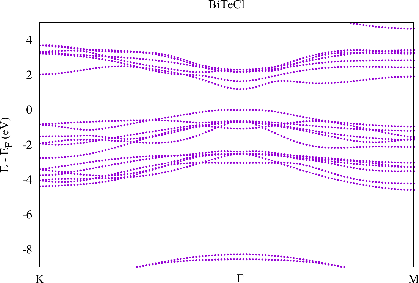
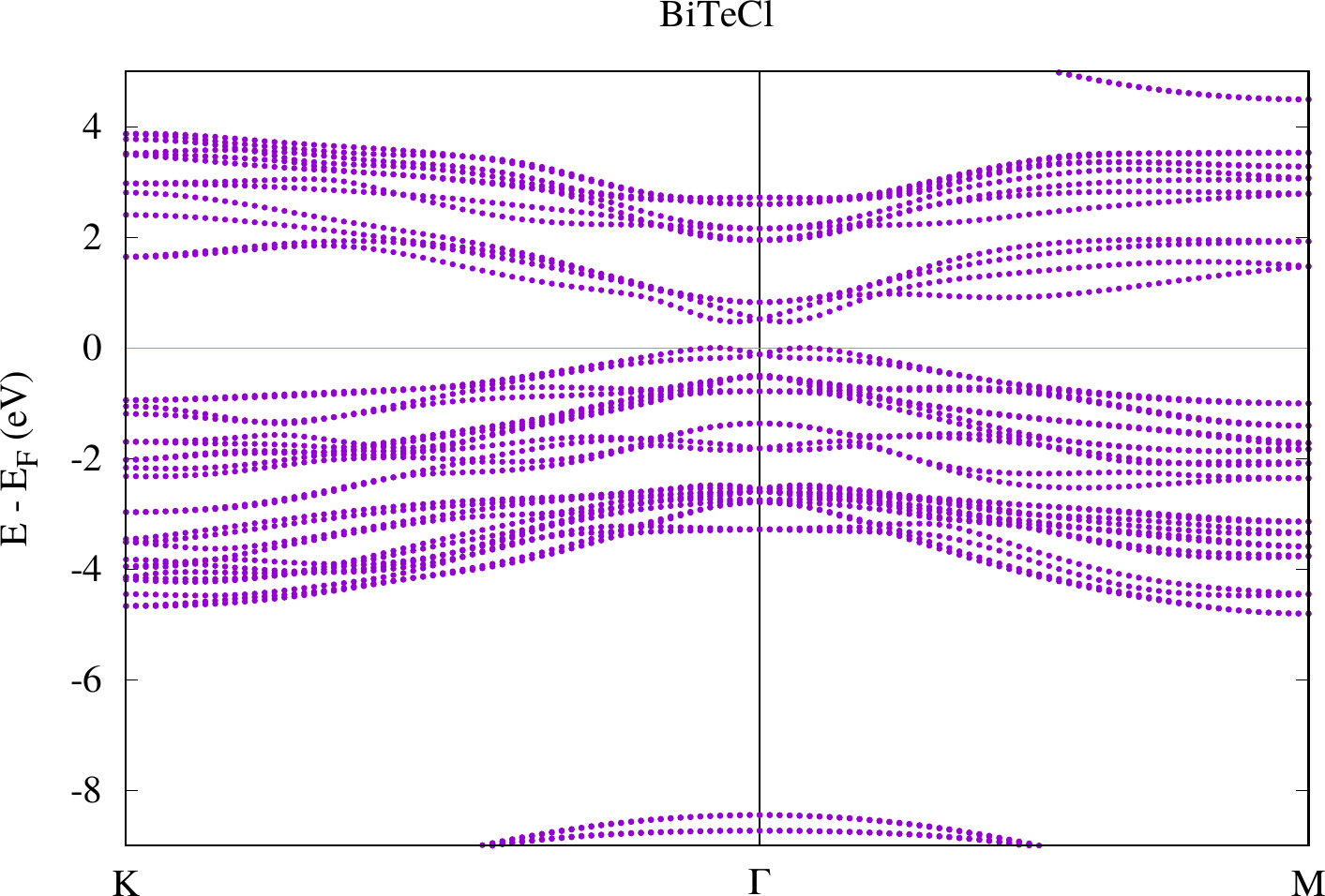
Compare the two plots. You should observe differences at the gamma point in the bands defining the band gap. For the case with SOC there actually is a spin-dependent band splitting where the states for one spin can be found at and those for the other spin at . We don't see the spin in this plot because we made a non-spinpolarized calculation. Otherwise this can also be highlighted with the weights that are stored in the banddos.hdf file.