
Calculating Green's functions
This tutorial explains how to set up Green-function calculations in FLEUR, how to choose a contour,
how to define onsite and intersite elements, what the main output quantities mean, and how the
resulting data can be used later for quantities such as Jij.
1. Basic idea
The Green-function functionality in FLEUR provides orbital-resolved and site-resolved propagators derived from the Kohn-Sham states of a converged calculation. Instead of solving a separate Green-function equation directly in real space, FLEUR constructs the Green function from the spectral representation of the Kohn-Sham eigenstates,
Inside each muffin-tin sphere, the wave functions are expanded in the LAPW+LO basis and projected onto selected local orbital channels. Numerically, FLEUR first builds the imaginary part of the projected Green function on a real-energy mesh and then reconstructs the Green function on the chosen complex contour through a Kramers-Kronig transformation,
- a real-energy mesh on which the imaginary part is constructed,
- one or more complex contours on which the final Green function is evaluated,
- a definition of the orbital channels and shells to be calculated.
2. Minimal setup
A Green-function calculation is activated in the calculationSetup section through a greensFunction block, while the actual orbital channels are selected by one or more greensfCalculation tags in the species section.
Contour setup
A minimal contour setup looks like:
<greensFunction l_mperp="F">
   <realAxis ne="5400" ellow="-1.0" elup="1.0"/>
   <contourSemicircle n="128" eb="-0.99" et="0.0" alpha="0.25"/>
</greensFunction>
The contour setup always has two parts:
- the global Green-function settings, which define the real-axis mesh,
- one or more contour definitions, from which you choose the contour appropriate for your calculation.
l_mperpenables spin-offdiagonal Green-function components for noncollinear calculations.neis the number of points on the real-energy mesh used to construct the imaginary part.ellowis the lower bound of the real-energy mesh.elupis the upper bound of the real-energy mesh.
ebis the real-energy starting point of a contour.etis the real-energy end point of a contour.labelis an optional name used to connect a contour to a specificgreensfCalculation.nis the number of contour points for contour types that use one point count.sigmais the imaginary offset used by contour types shifted off the real axis.
If several contour strategies are needed in one calculation, FLEUR allows multiple contour definitions:
<greensFunction l_mperp="F">
   <realAxis ne="5400" ellow="-1.0" elup="1.0"/>
   <contourSemicircle n="128" eb="-0.99" et="0.0" alpha="0.25"/>
   <contourRectangle n1="10" n2="128" n3="30" nmatsub="5" sigma="0.005" eb="-0.99" label="RectangleExample"/>
   <contourDOS n="5400" eb="-1.0" et="1.0" sigma="0.00314" analytical_cont="T" l_fermi="F" label="DOSExample"/>
</greensFunction>
The three standard contour choices are shown below.
1. Semicircle contour
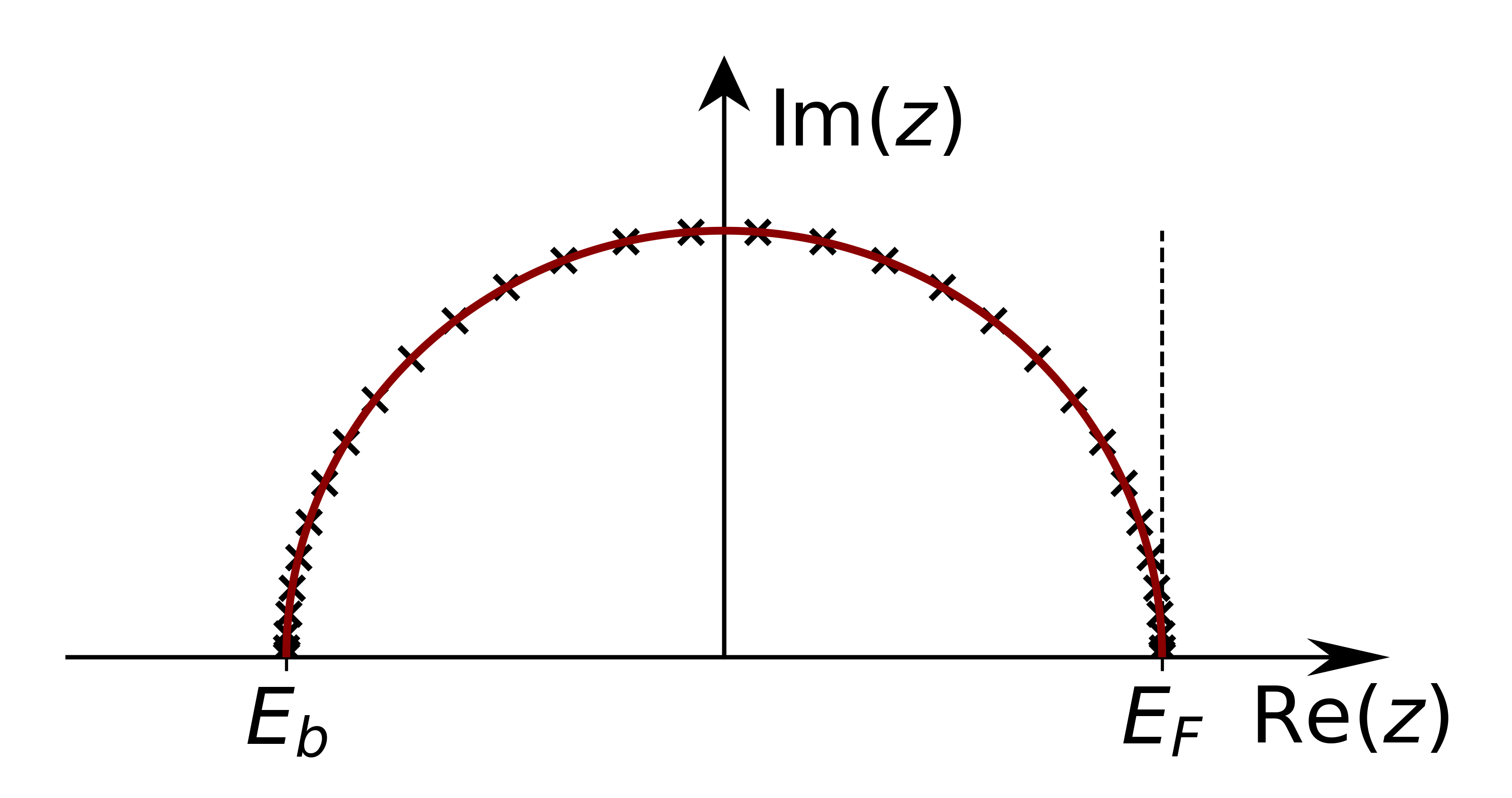
This is the standard default contour for many Green-function calculations.
Main extra parameteralphascales the imaginary height of the semicircle.
2. DOS contour
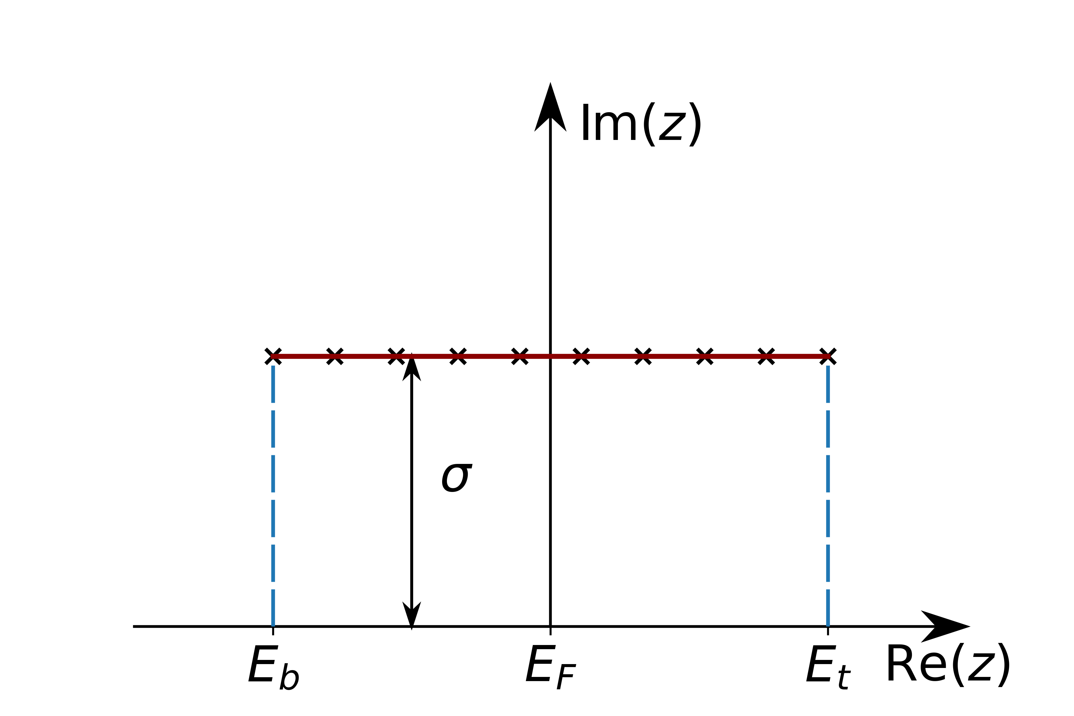
Useful for spectral quantities on a dense near-real-axis path.
Main extra parametersanalytical_contselects the analytical continuation form.l_fermicontrols whether the Fermi-function treatment is included.
3. Rectangle contour
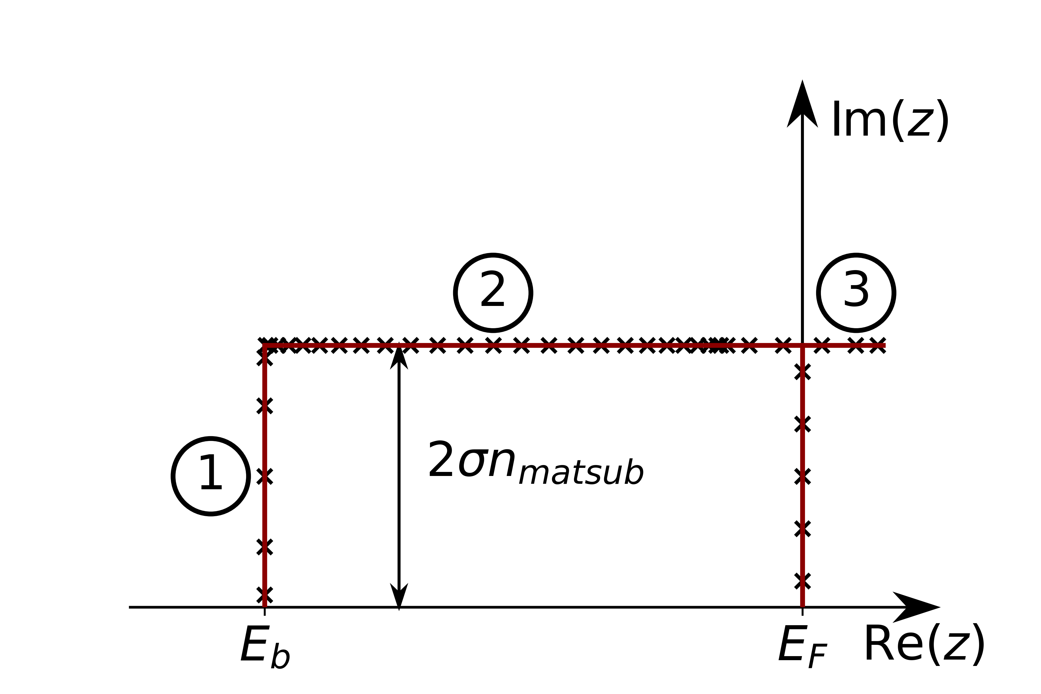
Useful when a Matsubara-like offset around the Fermi level is desired.
Main extra parametersn1is the number of points on the first vertical branch.n2is the number of points on the horizontal branch.n3is the number of points on the second vertical branch.nmatsubshifts the horizontal branch by integer Matsubara distances.
Element setup
The element setup specifies which orbitals should be calculated. The simplest onsite setup is:
<greensfCalculation l_sphavg="T">
   <diagElements s="F" p="F" d="T" f="F"/>
</greensfCalculation>
A first intersite setup for one shell is:
<greensfCalculation l_sphavg="T" nshells="1" kkintgrCutoff="d">
   <diagElements s="F" p="F" d="T" f="F"/>
</greensfCalculation>
l_sphavgisTfor spherically averaged Green functions andFfor radial-dependent Green functions.nshellsis the number of intersite shells to construct.kkintgrCutoffselects the cutoff strategy for the Kramers-Kronig integration.labelconnects this element setup to a named contour such asRectangleExampleorDOSExample.diagElementsselects onsite diagonal orbital channels through thes,p,d, andfswitches.
3. Typical workflow
- Start from a working FLEUR input for the system of interest.
- Add a
greensFunctionblock with a sensible real-energy mesh and one or more contours. - Add
greensfCalculationtags to the species or atom groups of interest. - Run FLEUR.
- Inspect the generated Green-function output, typically
greensf.hdf.
- Check the number of bands (
numbands) carefully. - Check the upper real-axis energy limit (
elup). - Check the density of the
k-point mesh. - Check the Brillouin-zone integration mode.
For smooth spectra in bulk calculations, the tetrahedron method is often the best starting point. Histogram mode can still be useful for tests or direct comparison with reference setups.
4. Output quantities
The most important Green-function-related outputs are:
| Quantity | Meaning |
|---|---|
sphavg |
Spherically averaged projected Green function. |
uu, dd, ud, du |
Radial channel data available when l_sphavg="F". |
mmpmat |
Occupation matrix obtained from contour integration. |
The occupation matrix is obtained from
The diagonal elements describe orbital occupations, while the offdiagonal elements describe orbital mixing and coherence between local orbitals.
5. Recommended example inputs
testing/inputfiles/greens/
Fe_bcc_GreensFunction— simplest bulk onsite, spin-diagonal, spherically averaged Green function.GreensFunctionRadial— comparesl_sphavg="T"andl_sphavg="F".GreensFunction_IntersiteSingleShell— first intersite shell.GreensFunction_IntersiteMultipleShells— several intersite shells.GreensFunction_MultiContour— several contours in one calculation.GreensFunction_mperp_xdir— noncollinear spin-offdiagonal Green function.GreensFunction_mperp_ydir— second noncollinear spin-offdiagonal example.
6. Application: Exchange parameters
One important application of the Green function is the calculation of intersite exchange parameters . These quantities describe how strongly the magnetic moments on sites and are coupled. They are useful for analyzing magnetic interactions, constructing Heisenberg models, and comparing first-principles results with spin-model simulations.
- The Green function gives direct access to onsite and intersite orbital propagation between magnetic atoms.
- These intersite matrix elements can be combined with exchange splittings to obtain pairwise exchange couplings.
- This is especially useful when shell-resolved magnetic interactions are needed.
For automated workflows, data provenance, and postprocessing, one can use
AiiDA-FLEUR documentation
to calculate Jij from the Green-function output in a reproducible workflow environment.