
1. Density of states
Besides the band structure, the density of states (DOS) also provides a direct view on the electronic structure of a material. It is easy to construct it from a DFT calculation. The difference is that while in a band structure the displayed data is k-point dependent, in a DOS an integration over the Brillouin zone took place.
1.1. Density of states for Si
We perform our first DOS calculations for Si. This starts by obtaining a self-consistent density with an 8x8x8 k-point mesh generated with
inpgen -inp.xml -kpt grid=8,8,8
as it is typically also generated with the default parameters (also use the other default parameters). We construct three different density of states on top of this calculation. Consider creating subfolders for each of them and copy the results (including the cdn.hdf file) of your self-consistent calculation to each subfolder.
To construct a DOS the inp.xml file has to be modified by setting output/@dos to "T".
There are also some parameters specified in the output/bandDOS XML tag. They have the following use: With minEnergy and maxEnergy the energy window for the
DOS is specified, with sigma one defines a broadening for each state to obtain a smooth result. By default sigma is 0.015. The three
different DOS calculations will use different values for sigma: 0.015, 0.005, 0.0015
Perform the three different DOS calculations on top of the already converged result (don't forget to select the correct k-point set).
The calculations will generate a Local.1 file,
where the "1" relates to the spin. In spin-polarized calculations also a Local.2 file will be generated (and for bandstructure
calculations a bands.2 file). The Local.1 file is a readable text file with several columns. The first column defines an energy mesh.
The second column is the total DOS and afterwards there are multiple columns for the projection of the DOS onto certain regions in
the unit cell and onto certain orbital characters around each atom. We are interested in the energy mesh, the total DOS, and the (column 5)
and (column 6) projections at the Si atoms. It may also be interesting to plot the DOS in the interstitial region (column 3).
Generate for each of the three calculations plots showing the total DOS, -, and -projected DOS, each. The plots should feature on the y axis the energy and on the x axis the DOS. They should look similar to what is displayed in the following figure.
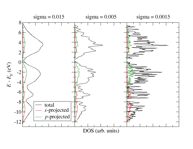
Comparison of DOS calculations with different sigma parameters for Si.
As an alternative you can also use the data stored in the banddos.hdf file to plot the DOS. Example Python scripts for extracting this
data are provided in the respective section of the Fleur user guide. If you want to use these
scripts you have to adapt them to your use case.
In combination with a bandstructure plot you can partially relate certain bands to the respective orbital character. Comparing the plots with each other you can observe results strongly varying with respect to the local Gaussian averaging according to the specified sigma parameter. Obviously it is crucial to find a sigma that provides a good balance between a smoothing of the curves and a resolution of the features of the electronic structure.
Of course, besides sigma, the smoothness of the curves also depends on the -point set. After all the density of states is obtained on the basis of the eigenstates at each point. The Gaussian averaging is needed because the -point mesh is not infinitely dense. For the smallest sigma (0.0015) we will therefore also test other -point sets. It should be enough if this is performed on top of the already obtained self-consistent density for the coarser -point mesh. Test
inpgen -inp.xml -kpt grid=23,23,23
and
inpgen -inp.xml -kpt grid=47,47,47
for the DOS calculation (it may take a while to generate the latter k-point list). How does it affect the result? How does it affect the computational demands? Your results should be similar to what is sketched in the following figure.
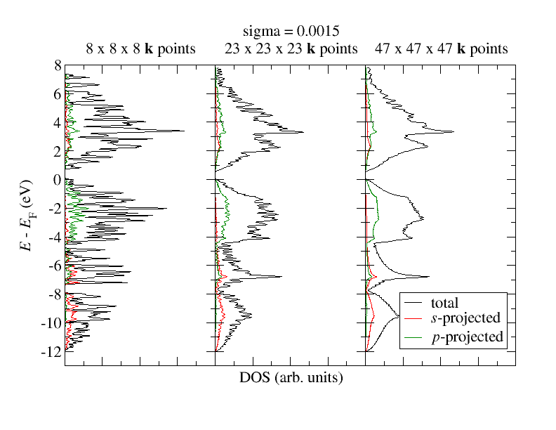
Comparison of DOS calculations for with different -point meshes for Si.
For the finest -point mesh: Do you think that we still see artifacts of the sigma parameter and the finiteness of the -point mesh in the plot? If so: Where in the plot is this most visible and why is it most visible in that region of the plot?
Note: There also is another mode to calculate a DOS with less demands on the k-point set. This is the tetrahedron method that introduces an interpolation scheme for the bands in the Brillouin zone. We will not investigate this approach here, but one should be aware that it also has shortcomings: For the interpolation the approach needs to know to which state at a given k-point some state at another k-point is connected. The naive assumption here is that the i-th state is connected to the i-th state, i.e., the possibility of band crossings is neglected. The approach can thus lead to artificial gaps.
2. Exercises
2.1. Band structure and DOS of a monatomic Cu wire (van Hove singularities)
Experimentalists are capable of producing monatomic wires of certain chemical elements, either on some substrate or free standing wires obtained with break junctions or by pulling scanning tunneling microscope (STM) tips out of a sample. For each energy the conductivity along such a wire is limited by the conductance quantum times the number of bands at the respective energy. Calculating the band structure of such a system therefore provides direct information on its ballistic electron transport properties.
We perform band structure and density of states calculations for a monatomic Cu wire. For this we set up a tetragonal unit cell with lattice parameters that provide a wide vacuum in two dimensions and the nearest neighbor distance between adjacent Cu atoms in the third dimension. Use and . For the self-consistent density calculation use a -point set generated with
inpgen -inp.xml -kpt grid=1,1,201
Note: Band structure calculations and DOS calculations are two different calculations. Even though both related flags can be set to 'T' in a single calculation without complaints of the code, most of the time it is not reasonable to do this. These calculations require -point sets with different properties. While a band structure calculation needs a -point path, a DOS calculation needs a -point set that nicely samples the whole volume of the (irreducible wedge of the) Brillouin zone.
For the band-structure calculation we explicitly generate the -point path by specifying "special k points" along the path:
inpgen -inp.xml -kpt band=100 -kptsPath "gamma=0,0,0;x=0.0,0.0,0.5"
Don't forget to select the hereby generated k-point list for the band structure calculation.
For the DOS calculation we use a very fine -point mesh such that the expected van Hove singularities at the band edges can easily be identified:
inpgen -inp.xml -kpt grid=1,1,7001
The number of energy mesh points for the DOS is fixed. As a consequence it is a good idea to refine the upper and lower limits of this mesh such that the mesh is not too coarse for our needs. Find out the Fermi energy obtained for the self-consistent density (grep -i fermi out) and adjust the energy window such that it only covers the interesting part of the band structure, e.g., from 0.1 Htr below the Fermi energy to 0.2 Htr above the Fermi energy. The energy window is specified by the parameters in 'output/bandDOS/@minEnergy' and 'output/bandDOS/@maxEnergy'. The sigma parameter should also be very small. Choose 0.0003.
Hint: Because of the large amount of k points this calculations takes a while. It may be advisable to employ some OpenMP parallelization to speed it up. For this execute in the terminal
export OMP_NUM_THREADS=4
before starting the calculation.
Plot the "total DOS" (column 2), the - (column 5), and the -projected (column 7) DOS. The van Hove singularities schould nicely be visible on every lower and upper band edge. Why is the -projected DOS so much smaller than the -projected DOS?
Results to be delivered: 1. The plot of the band structure, 2. The plot with the DOS.