
Extracting data from the banddos.hdf file
An important Fleur output file is the banddos.hdf file in which data relevant for the visualization and evaluation of band structures, density of states, and similar quantities is stored. Even though the employed HDF5 format is open, well documented, and coming with a large infrastructure of tools, working with such files might not be too intuitive. In this section some examples for extracting and working with the data from this file are sketched. The provided scripts are meant to be a guide for Fleur users. Fleur users are free to use the scripts, adapt them to their needs, and extract certain sections from them as an ingredient for their own scripts.
Note that the infrastructure around the HDF5 file format is very versatile. There are command line and graphical programs for directly inspecting and manipulating such files, as well as software libraries for many programming languages enabling the user to work with such files with a high level of control.
In the examples we concentrate on the work with the banddos.hdf file with the Python programming language, employing the masci-tools library. This library contains a lot of utility/IO and plotting functions specific for the Fleur code. For processing the banddos.hdf file the masci-tools library uses the h5py library. This is a very convenient way of working with HDF5 files. For plotting the scripts use the matplotlib library. Note that this library needs access to a graphical system, even if it is only used to write the plots to image files. For numerical postprocessing of the data stored in the banddos.hdf file, the scripts also use the numpy library.
Contents of the banddos.hdf file
Different Fleur calculations produce banddos.hdf files with differing contents. There may be DOS data stored in it or band-structure data. There may also be additional data in the form of weights stored in the file. To get a quick overview on what is stored in a banddos.hdf file one can use the command-line tools h5ls and h5dump, which are part of the HDF5 library. Invoking
h5dump -n 1 banddos.hdf
gives a list of groups (similar to directories in file systems), datasets (e.g., arrays), and attributes (typically simple variables and similar) stored in the file, Invoking
h5ls -r banddos.hdf
additionally provides information on the dimensions of the data sets but leaves away information on the attributes.
Of course, these tools can also be used to display values stored in the attributes and datasets.
An example of a graphical tool to browse the contents of HDF5 files is HDFView. This program can also be used to extract parts of the stored data in terms of multi-column text files.
Examples
The Bandstructure/DOS plotting functions in the masci-tools library are used in two steps. First we read in the provided banddos.hdf file and transform the data in a predictable way. The following code block shows the reading of a banddos.hdf file from a bandstructure calculation
from masci_tools.io.parsers.hdf5 import HDF5Reader
from masci_tools.io.parsers.hdf5.recipes import FleurBands

with HDF5Reader('banddos.hdf') as h5reader:
    data, attribs = h5reader.read(recipe=FleurBands)
The recipe defines what data is read in and how it is transformed. This encompasses things like shifting the eigenvalues so that the Fermi energy is at , converting them to eV and flattening everything into a one dimensional list.
After the data is read in it is put into two python dictionaries
data: This dictionary contains the data ready to plot and can be directly converted to a dataframe, if necessary, using thepandaslibrary for exampleattribs: Contains data related to the plot like labels and positions of special kpoints or the Fermi energy for example
At this point custom transformations or conversions can also be applied. In the second step we call one of two custom plotting functions. plot_fleur_bands or plot_fleur_dos, which provide standard visualizations for bandstructure and DOS calculations respectively.
Example 1: Plotting a band structure with orbital projection
This example is made for files created by Fleur band-structure calculations. It assumes that the banddos.hdf file is in the working directory. It reads it in and plots a band structure with a visualization of the projection of the eigenstates onto the character within the MT sphere of the first atom type. The bandstructure is then stored as an image in the file bandstructure.png.
from masci_tools.io.parsers.hdf5 import HDF5Reader
from masci_tools.io.parsers.hdf5.recipes import FleurBands

from masci_tools.vis.fleur import plot_fleur_bands

filepath='banddos.hdf'

with HDF5Reader(filepath) as h5reader:
    data, attributes = h5reader.read(recipe=FleurBands)

# We are interested in each state's d-projection in the MT sphere of the 1st atom type.
weightName = "MT:1d"
# Some other weights:
# weightName = "MT:1s" # s-projection in the 1st atom type's MT sphere.
# weightName = "MT:1p" # p-projection in the 1st atom type's MT sphere.
# weightName = "MT:1f" # f-projection in the 1st atom type's MT sphere.
# weightName = "MT:2s" # s-projection in the 2nd atom type's MT sphere (if available).

# Plot the bandstructure and save to a file bandstructure.png
# If we just want a unweighted bandstrcture, we can omitt the weight argument here
plot_fleur_bands(data, attributes,
                 weight=weightName,
                 limits={'y': (-10, 5)},
                 save_options={
                     'transparent': False,
                 },
                 show=False, #Change show to True to show the plot in a window
                 save_plots=True)
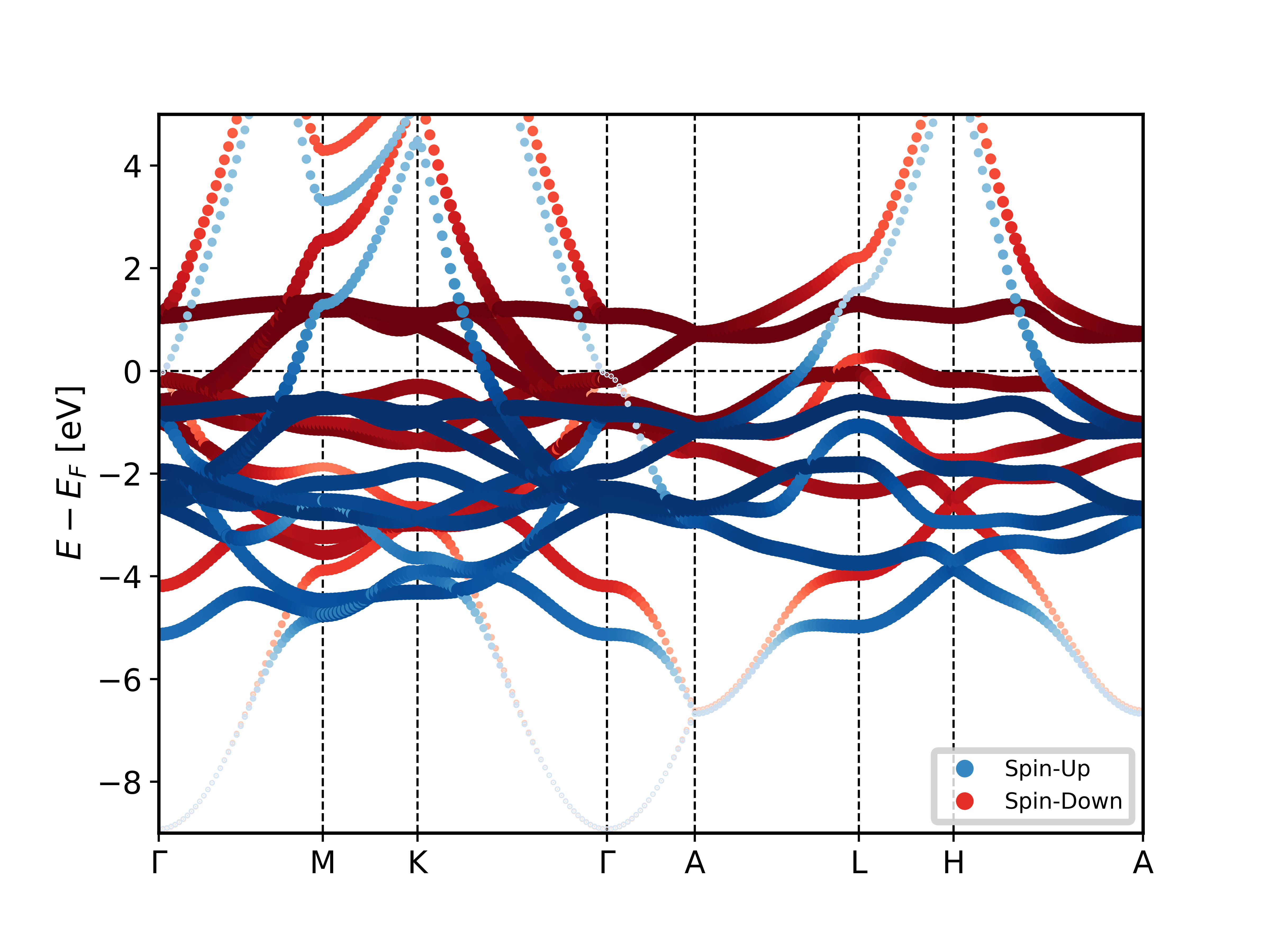
Using the script on a banddos.hdf file from a Fleur band structure calculation on an hcp Co unit cell results in the following plot of the related band structure.
Example 2: Plotting a DOS with orbital projection
This example is made for banddos.hdf files created by Fleur density of states (DOS) calculations. It assumes that the banddos.hdf file is in the working directory. It opens it and plots a DOS with a visualization of the projection of the DOS onto the character within the MT sphere of the first atom type. The DOS is then stored as an image in the file DOS.png.
from masci_tools.io.parsers.hdf5 import HDF5Reader
from masci_tools.io.parsers.hdf5.recipes import FleurDOS

from masci_tools.vis.fleur import plot_fleur_dos

filepath='banddos.hdf'

with HDF5Reader(filepath) as h5reader:
    data, attributes = h5reader.read(recipe=FleurDOS)

# Store the plot as an image to the file DOS.png
plot_fleur_dos(data, attributes,
               show_interstitial=False,
               show_atoms=None,
               plot_keys=['MT:1d'],
               xyswitch=True,
               limits={'energy': (-9,5)},
               legend_options={'loc':'lower right'},
               show=False,
               save_plots=True,
               save_options={
                     'transparent': False,
               },
               saveas='DOS')

#Choice for second example
#plot_fleur_dos(data, attributes,
#               show_atoms=None,
#               plot_keys=['MT:2p','MT:2d','MT:1s'],
#               limits={'energy': (-5,9)},
#               xyswitch=True,
#               show=False,
#               save_plots=True,
#               saveas='DOS',
#               save_options={
#                    'transparent': False,
#               },
#               legend_options={'loc':'lower right'})
Using the script on a banddos.hdf file from a Fleur DOS calculation on an hcp Co unit cell results in the left DOS plot of the following figure. Using it with the indicated modifications on a rock-salt NaCl unit cell results in the right plot.
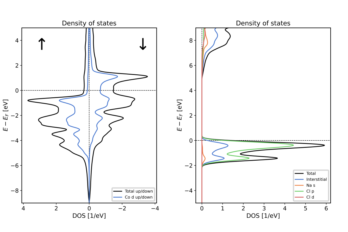
Total DOS of hcp Co (left) and rock-salt NaCl (right) together with contributions from different regions and different orbital character. Note that the Co unit cell contains two symmetry equivalent atoms. The DOS from the MT sphere of such an atom only covers one of the atoms. For NaCl it is visible that the valence band is dominated by states in the Cl MT sphere, while the lower edge of the conduction band features Na character. The states in the Na atoms reach far beyond the Na MT sphere, giving rise to large DOS contributions from the interstitial region and also to some Cl -like DOS.
Example scripts without masci-tools
All the previous examples can of course also be done without the masci-tools library, if you need really low-level access. In the following we show the same examples done in an explicit way.
Example 1: Plotting a band structure with orbital projection
This example is made for files created by Fleur band-structure calculations. It assumes that the banddos.hdf
file is in the working directory. It opens it and plots a band structure with a visualization of the projection of
the eigenstates onto the character within the MT sphere of the first atom type. On top it plots a band structure
without any highlighting in a slightly darker color. The bandstructure is then stored as an image in the
file bandstructure.png and as a vector graphic in the file bandstructure.svg.
The Python script used in this example is shown below. Note that this script is not optimized for performance. For
large banddos.hdf files this is very noticable. It is intended to demonstrate basic access to the data
stored in the banddos.hdf file. In detail it accesses
- The number of k points in
/kpts/@nkptand their (internal) coordinates in/kpts/coordinates. - The reciprocal Bravais matrix stored in
/cell/reciprocalCell. - The Fermi energy from either the last SCF iteration before performing the band-structure calculation or - if available - from the correction of the Fermi energy as indicated by the Fleur terminal output. This is stored in
/general/@lastFermiEnergy. - The indices and labels of the high-symmetry points of the -point path in
/kpts/specialPointIndicesand/kpts/specialPointLabels. - The eigenvalues to be plotted in the band structure in
/Local/BS/eigenvalues. - The weights for the projection of the eigenvalues to the character within the MT spheres of the st atom type stored in
/Local/BS/MT:1d. - The number of spins (1 for nonmagnetic, 2 for magnetic) in the calculation stored in
/general/@spins.
import math;
import numpy;
import h5py;
import matplotlib.pyplot as plt

##############################################################
# Open the banddos.hdf file and name some data groups in it. #
##############################################################
banddosFile = h5py.File('banddos.hdf', 'r')

cellData = banddosFile['cell']
kptsData = banddosFile['kpts']
generalData = banddosFile['general']
localData = banddosFile['Local']

#########################################################################################
# Generate x coordinates for each k point on the k-point path. For this the distance    #
# vector between adjacent k points is calculated and multiplied with the reciprocal     #
# Bravais matrix to transform from internal coordinates to cartesian coordinates. On    #
# this basis the distance between the two adjacent points is computed. The x coordinate #
# is the cumulative path length up to the respective point.                             #
#########################################################################################
xCoords = [0.0 for i in range(kptsData.attrs["nkpt"][0])]
for i in range(1,kptsData.attrs["nkpt"][0]):
   distVec = numpy.matmul(cellData["reciprocalCell"][0:3][0:3],
                kptsData["coordinates"][i][0:3] - kptsData["coordinates"][i-1][0:3])
   distance = math.sqrt(distVec[0]*distVec[0]+distVec[1]*distVec[1]+distVec[2]*distVec[2])
   xCoords[i] = xCoords[i-1] + distance
pathLength = xCoords[kptsData.attrs["nkpt"][0]-1]

###################
# Initialize plot #
###################
minY = -9.0
maxY = 5.0
figure = plt.figure()
axes = figure.add_subplot(1, 1, 1)
axes.set_xlim(xmin=0.0,xmax=pathLength)
axes.set_ylim(ymin=minY,ymax=maxY)
axes.set_ylabel("$E - E_\mathrm{F}$ (eV)")

####################################################################################
# Generate x axis tick labels together with coordinates and plot vertical lines at #
# these coordinates. Also plot a horizontal line to indicate the Fermi level       #
####################################################################################
scfFermiEnergy = generalData.attrs["lastFermiEnergy"][0]
tickLabels = ["uninitialized" for i in range(len(kptsData["specialPointIndices"]))]
tickCoords = [0.0 for i in range(len(kptsData["specialPointIndices"]))]
tickCoords[len(kptsData["specialPointIndices"])-1] = pathLength
for iSpecialPoint in range(len(tickLabels)):
   tickLabels[iSpecialPoint] = kptsData["specialPointLabels"][iSpecialPoint].decode('utf-8')
   # Every tick label that starts with a "g" or "G" indicates the Gamma point. The
   # respective tick label now gets replaced by a fitting Latex expression.
   if tickLabels[iSpecialPoint].lower().startswith('g'):
      tickLabels[iSpecialPoint] = "$\Gamma$"
plt.plot([0.0, pathLength], [0.0, 0.0], color='cyan', linestyle='-',
         linewidth=1.0, zorder=1)
for iSpecialPoint in range(1,len(kptsData["specialPointIndices"])-1):
   tickCoords[iSpecialPoint] = xCoords[kptsData["specialPointIndices"][iSpecialPoint]-1]
   plt.plot([tickCoords[iSpecialPoint], tickCoords[iSpecialPoint]], [minY, maxY],
      color='black', linestyle='-', linewidth=1.0,zorder=1)
plt.xticks(tickCoords,tickLabels)

#######################
# Plot band structure #
#######################
colors = ['red','blue'] # different colors for different spins (band structure with weight-dependent point size)
colorsB = ['maroon','darkblue'] # different colors for different spins (band structure with fixed point size)

# We are interested in each state's d-projection in the MT sphere of the 1st atom type.
weightName = "MT:1d"
# Some other weights:
# weightName = "MT:1s" # s-projection in the 1st atom type's MT sphere.
# weightName = "MT:1p" # p-projection in the 1st atom type's MT sphere.
# weightName = "MT:1f" # f-projection in the 1st atom type's MT sphere.
# weightName = "MT:2s" # s-projection in the 2nd atom type's MT sphere (if available).

# In this band structure we want to highlight a certain orbital character of each
# eigenstate. The size of each point in the bandstructure plot is determined by
# this. We norm the weight with respect to the maximum of the considered weights.
# Note that such visualizations and norms depend on the purpose of the visualization.
# This may also be something completely different, e.g., a color coding, a different
# calculation of the point size, or a different norm.
maxWeight = numpy.max(localData["BS"][weightName]) # This is for the norm.
for iSpin in range(generalData.attrs["spins"][0]):
   eigValsX = []
   eigValsY = []
   eigValsSize = []
   for iKpt in range(kptsData.attrs["nkpt"][0]):
      for iEigVal in range(len(localData["BS"]["eigenvalues"][iSpin][iKpt])):
         # Shift energy eigenvalue with respect to SCF Fermi energy and convert it
         # from Hartree to eV. The choice of the Fermi energy may vary for different
         # types of materials. If the Fermi energy differs from that of the last SCF
         # iteration this would imply a need to adapt the shift.
         valInEV = (localData["BS"]["eigenvalues"][iSpin][iKpt][iEigVal] - scfFermiEnergy)
         valInEV *= 27.211
         # We choose the weight of the point according to the projection of the eigenstate
         # onto the d character in the MT sphere of atom type 1.
         weight = localData["BS"][weightName][iSpin][iKpt][iEigVal]
         pointsize = 1.0 + 10.0*(weight/maxWeight) # Calculation of the point size.
         # Plot the energy eigenvalue only if it is within the range of the plot. The
         # eigenvalues are stored in order of increasing energy.
         if valInEV < minY : continue
         if valInEV > maxY : break
         eigValsX.append(xCoords[iKpt])
         eigValsY.append(valInEV)
         eigValsSize.append(pointsize**2.0)
   plt.scatter(eigValsX,eigValsY,s=eigValsSize,c=colors[iSpin],marker='.',zorder=2);
   plt.scatter(eigValsX,eigValsY,s=1.0,c=colorsB[iSpin],marker='.',zorder=3);

############################################################
# Store the plot as an image to the file bandstructure.png #
# and as a vector graphic to the file bandstructure.svg    #
############################################################
plt.savefig('bandstructure.png',dpi=300)
plt.savefig('bandstructure.svg')

###########################################
# Alternatively show the plot in a window #
###########################################
#plt.show()
Using the script on a banddos.hdf file from a Fleur band structure calculation on an hcp Co unit cell results in the
following plot of the related band structure.
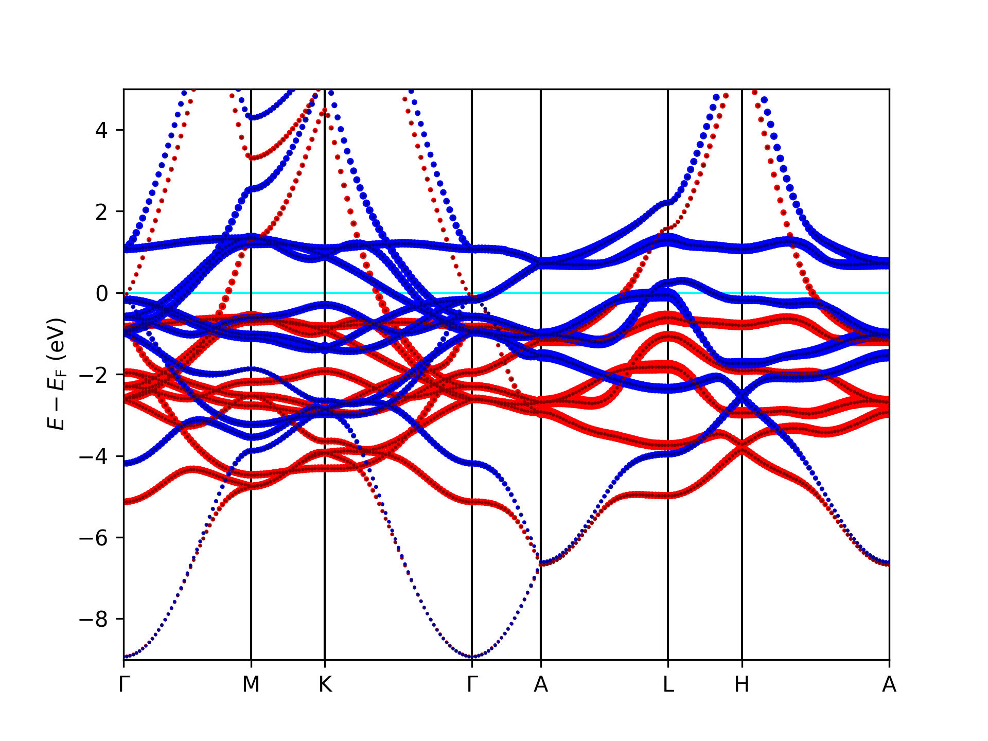
Band structure for hcp Co with projection onto the character in the MT sphere. The colors indicate the respective spin.
Example 2: Plotting a DOS with orbital projection
This example is made for banddos.hdf files created by Fleur density of states (DOS) calculations.
It assumes that the banddos.hdf file is in the working directory. It opens it and plots a DOS with
a visualization of the projection of the DOS onto the character within the MT sphere of the first
atom type. The DOS is then stored as an image in the file DOS.png and as a vector graphic in the
file DOS.svg.
The Python script used in this example is shown below. It accesses
- The number of spins (1 for nonmagnetic, 2 for magnetic) in the calculation stored in
/general/@spins. - The total DOS in states/Hartree as stored in
/Local/DOS/Total. - The 1st atom type's MT character contribution to the DOS stored in
/Local/DOS/MT:1d. - The energy grid (in Hartree relative to the Fermi level) on which the DOS values are provided as stored in
/Local/DOS/energyGrid.
import math;
import numpy;
import h5py;
import matplotlib.pyplot as plt

##############################################################
# Open the banddos.hdf file and name some data groups in it. #
##############################################################
banddosFile = h5py.File('banddos.hdf', 'r')

cellData = banddosFile['cell']
kptsData = banddosFile['kpts']
generalData = banddosFile['general']
localData = banddosFile['Local']

# Read in number of spins in the calculation. The plot should
# feature two panels for two spins and a single panel for
# a nonmagnetic calculation.
nSpins = generalData.attrs["spins"][0]

###################
# Initialize plot #
###################
minY = -9.0 ; maxY = 5.0
#minY = -5.0 ; maxY = 9.0 # choice for 2nd example

if nSpins == 2:
   figure, axes = plt.subplots(1, 2, sharey=True, figsize=(6, 6))
   figure.subplots_adjust(wspace=0.0)
else:
   axes = [1]
   figure, axes[0] = plt.subplots(1, 1, figsize=(4, 6))
   figure.subplots_adjust(left=0.2)

# Note: For nSpins==1 nSpins-1 is 0 and we do some things twice.
#       For 2 spins addressing indices 0 and nSpins-1 affects the
#       different subplots.
axes[0].set_ylim(ymin=minY,ymax=maxY)
axes[nSpins-1].set_ylim(ymin=minY,ymax=maxY)
axes[0].set_ylabel("$E - E_\mathrm{F}$ (eV)")
axes[0].set_xlabel("states / eV")
axes[nSpins-1].set_xlabel("states / eV")

############
# Plot DOS #
############
colors = ['black','red','blue','green','purple'] # different colors for different weights

# Select the weights of the DOS contributions to be plotted.
# We are interested in the total DOS and the d-like DOS in the MT sphere of
# the 1st atom type.
weightNames = ["Total","MT:1d"]
#weightNames = ["Total","MT:2p","MT:2d","MT:1s","INT"] # choice of weights for 2nd example
# Some other weights:
# weightName = "INT"   # DOS in the interstitial region
# weightName = "MT:1s" # s-like DOS in the 1st atom type's MT sphere.
# weightName = "MT:1p" # p-like DOS in the 1st atom type's MT sphere.
# weightName = "MT:1f" # f-like DOS in the 1st atom type's MT sphere.
# weightName = "MT:2s" # s-like DOS in the 2nd atom type's MT sphere (if available).

#####################################################################################
# Plot the DOS for the selected weights                                             #
# Note: 1. In the banddos.hdf file the energy grid is stored in Hartree relative to #
#          the Fermi energy. We transform that to eV.                               #
#       2. The DOS is stored in states/Hartree. We transform that to states/eV.     #
#####################################################################################
energies = localData["DOS"]["energyGrid"][:] * 27.211
for iSpin in range(nSpins):
   for iWeight in range(len(weightNames)):
      values = []
      values[:] = localData["DOS"][weightNames[iWeight]][iSpin][:] / 27.211
      minIndex = 0
      maxIndex = len(values)-1
      for i in range(len(values)):
         if energies[i] < minY: minIndex = i
         if energies[i] > maxY:
            maxIndex = i
            break
      axes[iSpin].plot(values[minIndex:maxIndex+1],energies[minIndex:maxIndex+1],
                       color=colors[iWeight],label=weightNames[iWeight],zorder=2)

##########################################################################################
# Do some postprocessing in the plot                                                     #
# 1. Norm the x axis of the two subplots for spin-polarized calculation.                 #
# 2. Plot a line to indicate the Fermi level.                                            #
# 3. Plot spin-indicating arrow symbols in the subplots for spin-polarized calculations. #
# 4. Put a legend in one of the subplots.                                                #
# 5. Invert the x axis in the left subplot for spin-polarized calculations.              #
##########################################################################################
xlims = [axes[0].get_xlim(),axes[nSpins-1].get_xlim()]
maxX = max(xlims[0][1],xlims[nSpins-1][1])
axes[0].set_xlim(xmin=0.0,xmax=maxX)
axes[nSpins-1].set_xlim(xmin=0.0,xmax=maxX)

axes[0].plot([0.0, maxX], [0.0, 0.0], color='cyan', linestyle='-',linewidth=1.0, zorder=1)
axes[nSpins-1].plot([0.0, maxX], [0.0, 0.0], color='cyan', linestyle='-',linewidth=1.0, zorder=1)

if nSpins == 2:
   spinArrows = [r"$\uparrow$",r"$\downarrow$"]
   for iSpin in range(nSpins):
      xlims = axes[iSpin].get_xlim()
      axes[iSpin].annotate(spinArrows[iSpin], [0.75*xlims[1],3.5],ha="center",va="center",size=24)

axes[nSpins-1].legend(loc='lower right')

if nSpins == 2:
   axes[0].invert_xaxis()
   axes[1].get_yaxis().set_visible(False)

##################################################
# Store the plot as an image to the file DOS.png #
# and as a vector graphic to the file DOS.svg    #
##################################################
plt.savefig('DOS.png',dpi=300)
plt.savefig('DOS.svg')

###########################################
# Alternatively show the plot in a window #
###########################################
#plt.show()
Using the script on a banddos.hdf file from a Fleur DOS calculation on an hcp Co unit cell results in the left DOS plot of the following figure. Using it with the indicated modifications on a rock-salt NaCl unit cell results in the right plot.
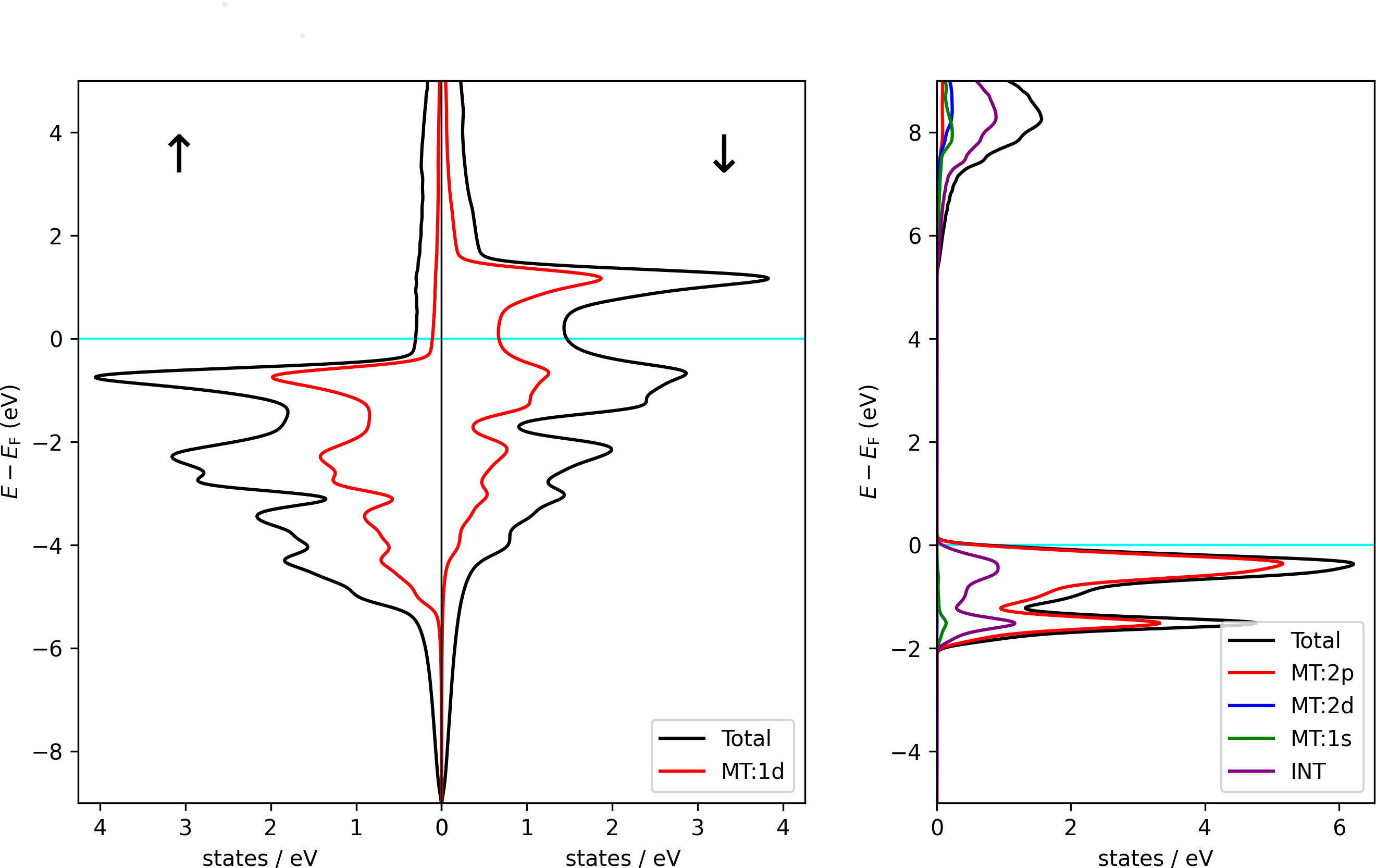
Total DOS of hcp Co (left) and rock-salt NaCl (right) together with contributions from different regions and different orbital character. Note that the Co unit cell contains two symmetry equivalent atoms. The DOS from the MT sphere of such an atom only covers one of the atoms. For NaCl it is visible that the valence band is dominated by states in the Cl MT sphere, while the lower edge of the conduction band features Na character. The states in the Na atoms reach far beyond the Na MT sphere, giving rise to large DOS contributions from the interstitial region and also to some Cl -like DOS.