
Overview
On the second day, we explore the features of FLEUR to describe magnetic states:
- Visualize the magnetization density of fcc Fe
- Calculate the energy difference between FM and AFM states
- The same using a non-collinear calculation
- The same using a spin-spiral calculation
- Calculate the magnetic anisotropy of an Fe monolayer from total energies
- Do the same with the magnetic force theorem
1. Magnetization density of fcc Fe
We start from an input file for fcc Fe with Cu lattice constant:
Fe fcc in Cu lattice constant
&input film=f /
&lattice latsys='cF' a0=6.82 /
1
26 0.0 0.0 0.0
and create the inp.xml file with the command
inpgen < inp_Fe
We observe that in the inp.xml-file now <magnetism> contains jspins=2 and in
the <species> line we find magMom=2.20. Here an
initial magnetic moment is given, if you have a better guess for the
magnetic moment, you can change this value now.
Now we create the starting density and converge the calculation as ususal.
Notice, that when you check the convergence (e.g. grep dist out)
you get a distance for spin 1 and spin 2, additionally for the charge and
magnetization density. Of course all these values have to be miminized.
After about 20-30 iterations this calculation is converged. You can now check
for the magnetic moment (e.g. grep mm out) and see, that it is roughly
2.59 Bohr. Keep in mind, that we calculate fcc Fe, not bcc which has a moment
of 2.20 Bohr!
As a final task, we plot the magnetization density. This is not very
different from plotting a charge density: in <plotting> set iplot=T, run
fleur and modify the plot_inp file that is created. If you run fleur again,
you now get a density for spin 1 and a density for spin 2, which you have to
subtract (e.g. in XCrysDen - disable 3D plotting in Virtual Box).
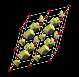
Magnetization density isosurface at -0.0028 e-/a.u. shows that the density turns negative in the interstitial region. Furthermore, the octahedral and tetrahedral voids of the fcc lattice are nicely visible.
2. Energy difference between FM and AFM states
2.1 collinear calculation
Now let's calculate energy difference between ferromagnetic (FM) and antiferromagnetic (AFM) fcc Fe from a collinear calculation. For this we have to choose at least a 2-atom unit cell, if the antiferromagnetic ordering vector is along the (cubic) [001] direction, a tetragonal unit cell with 2 atoms (one in the center, one in the corner, like in body centered tertagonal) will do.
Fe fcc 2-atom uc
&input film=f /
&lattice latsys='tP', a=0.7071068, c=1.0, a0=6.82 /
2
26 0.0 0.0 0.0
26 0.5 0.5 0.5
We start as usual a ferromagnetic calculation:
- generate an inp.xml file running inpgen
- iterate and converge to self-consistency
Now, you can check whether your magnetic moments are the same as in the Fe bulk
(fcc) collinear case. If not (by default you will get 2.606 Bohr), you can
increase the numbers of k-points in both cases, normally the spin moment
depends most sensitively on this parameter. Furthermore, you can see whether
the total energy (grep "on ener" out) is twice the number you got in the
primitive unit cell
(they will differ by about 0.058 mhtr in the default case, which is not bad).
Now you can proceed to calculate AFM bct Fe:
Fe fcc 2-atom uc
&input film=f /
&lattice latsys='tP', a=0.7071068, c=1.0, a0=6.82 /
2
26.0 0.0 0.0 0.0
26.1 0.5 0.5 0.5

&atom element="Fe" id=26.0 bmu=2.20 /
&atom element="Fe" id=26.1 bmu=-2.20 /
&end /
Proceed as above. Now, we can compare the magnetic moment and the total energy to the FM case:
- The moment went down from 2.61 Bohr (FM) to +/-1.78 Bohr in the AFM case.
- The total energy of the AFM state is only 0.55 mhtr (7.5 meV per Fe atom) higher than the FM state.
Neither state is the ground state. We will investigate this in the section with spin-spiral calculations.
2.2 Non-collinear calculation
The energy difference between FM and AFM fcc Fe can also be determined by a non-collinear calculation. This is of course computationally much more demanding, but allows you to investigate also other magnetic structures.
Suppose, the direction of the magnetization of an atom is described by two Euler angles alpha (polar angle) and beta (azimuthal angle). Then, the
- FM state is described by alpha=0 and beta=0 for both atoms, and the
- AFM state is described by alpha=0 and beta=π for the second one
and we can investigate the total energy as a function of the angle beta.
Start with the input-file for the input generator used in the AFM case but
invoke inpgen -noco < inp_Fe to generate an inp.xml file containing a few
more options for the non-collinear case.
In the inp.xml file, set noco=T and ctail=F and run fleur to reach
self-consistence. For better convergence, we further increase the basisfunction
cutoff to kmax=3.8 and gmax=11.4. You will realize that instead of cdn1
(or cdnXX) files
your charge density(matrix) is now stored in a file called rhomat_inp. When
you check charge density convergence, also a distance for "spin 3" is given,
that is the spin off-diagonal part of the density matrix.
After about 30 iterations the density is converged. Store the total energy,
remove the broyd* files (since 3.1: mixing_history) and now turn the
magnetization of one of the Fe atoms.
E.g. we could setting beta=0.1*Pi for the second atom, run another 15
iterations and save again the output and repeat this procedure until β=π.
Being are short in time and to avoid constrained spin-moment calculations, we
set beta=1.0*Pi immediately.
So, we create a new directory (say AFM), copy inp.xml, rhomat_inp and sym.out into this folder and run several iterations. After (rather slow) convergence, we see that the magnetic moment again dropped to +/- 1.76 Bohr (although it appears as positive values for both atoms, since β takes care of the minus sign) and the energy difference between FM and AFM amounts now to 10.5 meV per Fe atom. It's not exactly the same value as in the collinear calculation as it also allows for a non-collinear interstitial density.
2.3 Spin-spiral calculation
As a third possibility to calculate the energy difference between AFM and FM bct Fe, we try now a spin-spiral calculation. For this, we can start again from the primitive fcc unit cell. Since our AFM state can be described as spin-spiral proceeding in the (cartesian) z-direction, the spin-spiral vector has to be oriented in (1 1 0) direction in internal units:
 b  (-1  1  1)  (1)      (0)
 -  ( 1 -1  1)  (1) =  b (0)
 2  ( 1  1 -1)  (0)      (1)
When a spin-spiral with a q-vector q = (qx,qy,qz) is defined, the moment of an atom with internal coordinate t = (tx,ty,tz) is rotated by 2 π (q.t) around the z-axis. So it is easy to show, that a q-vector of (0.5, 0.5, 0.0) will lead to an AFM structure. But first, the moment of the atom has to be turned into the (x,y) plane, otherwise, a rotation around z has no effect.
Let's start with a collinear Fe fcc calculation. Since the spin-spiral lowers the symmetry of the fcc lattice (from cubic to tetragonal), we start from the input-generator again:
- add
&qss 1.0 1.0 0.0 /at the end of the inp_Fe-file for the input generator - running inpgen will produce inp.xml and sym.out files with the correct symmetry
- converge the non-collinear calculation as before (set β=π/2)
Save the results in some directory (e.g. q=0.0) and keeping just inp.xml,
sym.out and rhomat_inp continue with the AFM state by setting <qss> 0.5 0.5 0.0
</qss>. The energy difference finally obtained is 8.9 meV per Fe atom.
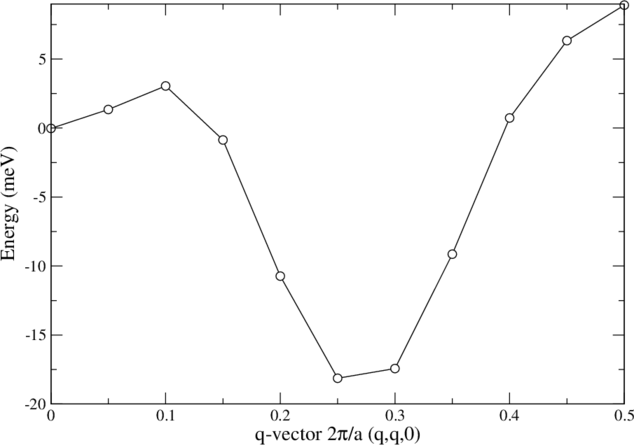
You can get the spin spiral dispersion by varying <qss> between 0.0 and 0.5.
3. Magnetocrystalline anisotropy of Fe monolayers
3.1 via total energy
This example shows the steps for a magneto-crystalline anisotropy energy (MAE) calculation for an Fe monolayer at the Ag(001) in-plane lattice constant by total energy calculations. The MAE is the energy difference between two (collinear) magnetic states with the spin-quantization axis (SQA) pointing in different directions. E.g. for a thin film, the magnetization could be perpendicular to the surface or parallel. This anisotropy is made up of two contributions:
- the classical dipole-dipole energy (not included in the total energies we calculate here, but can be added as soon as you know the magnetic moments), and
- the magnetocrystalline anisotropy energy, a spin-orbit coupling (SOC) effect. This is what we are interested in here.
The way we calculate with SOC, we lower the symmetry of our system . The
information about the direction of the SQA can already be included in the input
file for the input-generator. In terms of azimuthal (θ) and polar (φ) angle
perpendicular or parallel to the surface are (0.0, 0.0) or (π/2,0.0),
respectively. A general direction in between is e.g. (0.7, 0.0). Therefore, we
add in the last line if the input file &soc 0.7 0.0 /.
The next steps are:
- set
<soc theta="0.00000" phi="0.00000" l_soc="T" />in the inp.xml file - converge a calculation
- reuse cdn1 and sym.out from this calculation, but set theta="1.57080" in the inp.xml file converge again.
When you look for the magnetic moments ( grep mm out ), you will notice that you get now two numbers: spin and orbital moment:
| SQA | spin moment | orbital moment | total energy |
|---|---|---|---|
| z | 3.31 Bohr | 0.15 Bohr | -1272.7036994 htr |
| x | 3.31 Bohr | 0.11 Bohr | -1272.7036651 htr |
difference (MAE) 0.0000343 htr
While the spin-moments are identical, the orbital moments differ. The direction with the larger orbital moment is also the one with the lower total energy. This is consistent with a prediction from perturbation theory. The MAE is a tiny number, about 0.9 meV, but large as compared to MAEs of bulk systems. Although this result is not too bad, a convergence test w.r.t. the number of k-points is always in order for MAE calculations.
3.2 via force theorem
The force theorem states that MAE is given by the difference in band energies (sum of valence eigenvalues) obtained with spin-orbit coupling for two different spin-quantization axes, using the same self-consistent scalar-relativistic potential.
scalar relativistic calculation:
- use the inp.xml and sym.out file from above but with soc=F
- run fleur as usual
- coverge to self-consistency. The spin moment is again about 3.31 Bohr.
calculation with spin-orbit coupling:
- copy a set of the files: cdn1 inp.xml sym.out into two different directories
(e.g. oopl and inpl)
- go to oopl, set theta=0.00 and l_soc=T in the inp.xml file
- run fleur for a single iteration
- go to inpl, set theta=0.5*Pi and 1l_soc=T in the inp.xml file
- run fleur for a single iteration
- cd .. ; grep 'sum of eig' ./*pl/out
Now you have two numbers. The eigenvalue sum of 'oopl' is for the spin direction perpendicular to the surface (out-of-plane, we set θ=0 and φ=0). In 'inpl' (in-plane, θ= π/2 and φ=0) is the value for the magnetization in the surface plane ([100]-direction)
All you have to do now, is to subtract these numbers and you get the MAE! You will find that the easy axis of the magnetization is out-of plane and the MAE is 0.96 meV.
You will often get an error if the symmetry of your setup is broken by the spin-quantization axis. In case you do not break symmetries connecting quivalent atoms and you do not run more than a single iteration (itmax=1) you can still use the energies for the evaluation of the MAE if the k-point set corresponds to the broken symmetry.
4.0 LDA+U calculations
Finally, we test the application of the LDA+U method, which can help to describe strongly correlated materials more properly. E.g. NiO has in an LDA calculation a very small bandgap (0.4eV) and too small magnetic moment (1.2 Bohr). The LDA+U method cures these problems.
First we start with a GGA calculation (also GGA underestimates gap and moments): create the inp.xml file from inp_NiO:
NiO bct uc (AFM1)
&input film=f /
&lattice latsys='tP', a0=7.927, a=0.7071068, c=1.0  /
4
28.0 0.0 0.0 0.0
 8   0.5 0.5 0.0
28.1 0.5 0.5 0.5
 8   0.0 0.0 0.5
&atom element="Ni" id=28.0 bmu= 1.1 /
&atom element="Ni" id=28.1 bmu=-1.1 /
Now we could try to converge the GGA calculation, but this is rather unstable.
Therefore, we directly turn on LDA+U: Insert the parameters U and J (taken from
literature) in the inp.xml for the Ni species below the energy parameters and
above the line for the LO's:
<ldaU l="2" U="8.0" J="0.9" l_amf="F"/>
more information on this parameters you can find in the Fleur docu.
- set itmax="1" and run fleur
If you now check the convergence (grep dist out) you will see, that you find
also a distance of the density matrix. This matrix is stored in a file n_mmp_mat,
also residing in the working directory now. Since this information is now included
in the broyd* files (since version 3.1: mixing_history) for mixing:
- remove the broyd* (mixing_history) files
- set itmax="19" and run fleur again
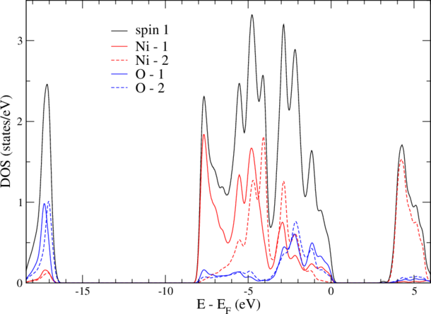
and find now also the density matrix converged. Since version 3.1 the mixing_history is automatically reset and n_mmp_mat is called n_mmp_mat_out. Now, the magnetic moment of NiO is large (1.8 Bohr) as it should be and also the gap is big (3.3eV). Notice, that in nature NiO has AFM II order, which we did not calculate here. For our calculation, the DOS should look like
Now, we can swich off the LDA+U again and see, what are the pure GGA values: 1.3 Bohr and a vanishing gap.