
Obtaining a density of states (DOS)
The calculation of a density of states (DOS) is based on the presence of a self-consistent density in the working directory. With this starting point two main adaptions have to be performed in the Fleur input file.
To enable the calculation of a DOS the switch output/@dos has to be set to T. Furthermore one of
several DOS calculation modes has to be selected by setting the output/densityOfStates/@ndir parameter
to the respective value. : Calculate a DOS and stop the program without generating a new density; :
Create a DOS in the last iteration of an SCF run; : Calculate an orbital decomposition of the DOS, too.
The output of a DOS calculation depends on several parameters. Most important is the range of the energy mesh on which the DOS is calculated.
The range of the energy mesh is specified by the two parameters output/densityOfStates/@minEnergy
and output/densityOfStates/@maxEnergy which have to be provided in . To get an estimate on
a possibly required offset it is a good idea to check the value of the Fermi energy with grep FermiEnergy out.xml.
The generation of a DOS relies on the chosen k point set used to sample the Brillouin zone. Since this is always finite the contributions comming from each calculated state have to be broadened in energy to avoid the calculation of an overly spikey DOS that is mainly an artifact of the Brillouin zone sampling. For this the DOS is convoluted with a Gaussian distribution.
The Gaussian is specified in terms of the standard deviation in output/densityOfStates/@sigma.
Note that the optimal choice of the standard deviation depends on the fineness of the -point mesh and also on material properties like the dispersion of the bands in the chosen energy range. The choice of the parameter therefore cannot be done automatically but is a task for the user. A too small yields an overly spikey DOS while a too large yields an overly smooth DOS that does not show any details. The following figure demonstrates this interrelation. It shows the total DOS for Si as well as the projections of the DOS onto the and states in one of the MT spheres. For the construction of the DOS the left plot uses the default parametrization, while the other two plots modify the parameter and the -point mesh for the DOS calculation (not for the SCF run).
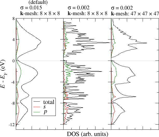
DOS for Si with different parameters.
It can be seen that the default sigma parameter here yields an overly smooth DOS that abstracts from the details. Not even the band gap can be estimated in this way. When reducing the parameter the DOS becomes very spikey because the -point density is too low to actually resolve a DOS on such a fine energy mesh. Only a reduction of together with an increase of the -point density yields a DOS that is not overly spikey but resolves the details of the electronic structure. But even in this plot the -point density is not high enough to completely overcome the spikes in the range of the unoccupied bands. Of course, it is expected that such artifacts especially show up in the range of the unoccupied bands because the dispersion for unoccupied bands is typically larger than for occupied bands.
The DOS can also be obtained by employing the so called tetrahedron method for Brillouin zone integration. In this method the irreducible wedge of the Brillouin zone is decomposed into small tetrahedra. The eigenvalues and all related properties are only obtained at the corners of each tetrahedron. Then the eigenvalues are linearly interpolated inside the tetrahedron.
The tetrahedron method is enabled by setting the calculationSetup/bzIntegration/@mode keyword to tria. This changes the -point
generation to the desired mode. As this mode is not based on a Monkhorst-Pack-grid, the XML element kPointCount should be
used to specify the number of -points.
The following figure demonstrates the effect of this method on the DOS. Both calculations use the same charge density and the same number of -points inside the irreducible brillouin zone.
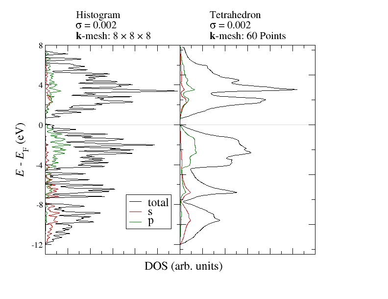
DOS for Si with histogram and tetrahedron method.
The differences between the above used histogram method and the tetrahedron method can be seen very clearly. Already with the relatively small amout of -points the DOS obtained from the tetrahedron method shows very clear features similar to the DOS with the high -point density above.
The main output of a DOS calculation is the file DOS.1 for nonmagnetic calculations and an additional file DOS.2 for
the second spin in spin-polarized calculations. These files consist of multiple columns of values, where the first column provides
the energy and all other columns provide projected DOS values. In short form the order of the columns is
(energy, total DOS, interstitial DOS, vacuum 1 DOS, vacuum 2 DOS, (for each atom type: DOS in MT), (for each atom type: (for l=0..3: l projected DOS in MT))).