Plotting densities

The FLEUR code offers several options of plotting the input density as a post-process calculation after a successful self-consistency run. The corresponding switches can be found in the output section of the Fleur input file under

<plotting iplot="0" score="F" plplot="F"/>

When setting the parameter to 2 starting Fleur will print out a warning, saying there is no plot_inp file. It also generated a prototype of this file. The score switch determines whether or not the core electron charge should be subtracted, so only the valence electron density will be plotted. plplot is currently without function.

In the plot_inp file, the various plotting options can now be specified. An example file looks as follows (warning: the file is partially fixed format and should be edited with care!):

 2,xsf=T,polar=F
 &PLOT twodim=t,cartesian=t
   vec1(1)=10.0 vec2(2)=10.0
   filename='plot1' /
 &PLOT twodim=f,cartesian=f
   vec1(1)=1.0 vec1(2)=0.0 vec1(3)=0.0
   vec2(1)=0.0 vec2(2)=1.0 vec2(3)=0.0
   vec3(1)=0.0 vec3(2)=0.0 vec3(3)=1.0
   grid(1)=50  grid(2)=50  grid(3)=50
   zero(1)=0.0 zero(2)=0.0 zero(3)=0.5
   filename ='plot2' /

The first number in the first line gives the number of plots to be made. Each plot then has some individual options. The two other global options are xsf (here: true), which specifies the type of output file. T will produce .xsf files for XCrySDen and F gives simple tabular files with the coordinates and output variable (e.g. $\rho(\vec{r})$) in several columns. polar enables 3 additional plots of the magnetization density amplitude $|m|$ and polar angles $\theta$ and $\phi$. This is only relevant for calculations with non-collinear magnetism.

The other switches set plot-specfic options.

• twodim: Determines whether a 2-dimensional or 3-dimensional density plot is created.
• cartesian: Are the following options given in internal or cartesian (Bohr radii) units?
• vecN(i): Bravais matrix of the system in question.
• grid(i): Number of grid points in each direction.
• zero(i): Origin shift of the plot.
• filename: Name of the files if xsf is false.

If one of the options is not specified, FLEUR will use default options hardcoded into the plotting routine:

• twodim=T
• polar=F
• cartesian=T
• grid(i)=100 for each direction
• vecN(i)=zero(i)=0 for each direction and entry in the Bravais matrix.
• filename='default'

To better understand which files are written, here are some examples for the case of a single 3D plot with xsf=T:

• non-spinpolarized: plot.xsf with a single DATAGRID containing the data.
• collinear: plot.xsf with two DATAGRID blocks (spin-up and spin-down density).
• non-collinear: cdn.xsf, mdnx.xsf, mdny.xsf, mdnz.xsf with two DATAGRID blocks each (2nd one is redundant).
• non-collinear with polar=T: cdn_pl.xsf, mdnx_pl.xsf, mdny_pl.xsf, mdnz_pl.xsf, mabs_pl.xsf, mtha_pl.xsf, mphi_pl.xsf with two DATAGRID blocks each (2nd one is redundant).

The non-colinear cases yield three additional density files for the magnetization density in each direction, e.g., mdnx.hdf and so on.

The following shows two plots created for a converged calculation on collinear ferromagnetic $\text{Fe}_2 \text{N}$. They were obtained in XCrySDen by reading in the plot.xsf and setting the multiply Factor under Tools -> Data Grid to $1.0$ for the spin-up density (DATAGRID #0) and to $\pm 1.0$ for the spin-down density (DATAGRID #1) to obtain the total density and magnetization density respectively.

The first plot shows an isosurface for a certain charge density value on top of the structure extended to two unit cells in y- and z-direction.

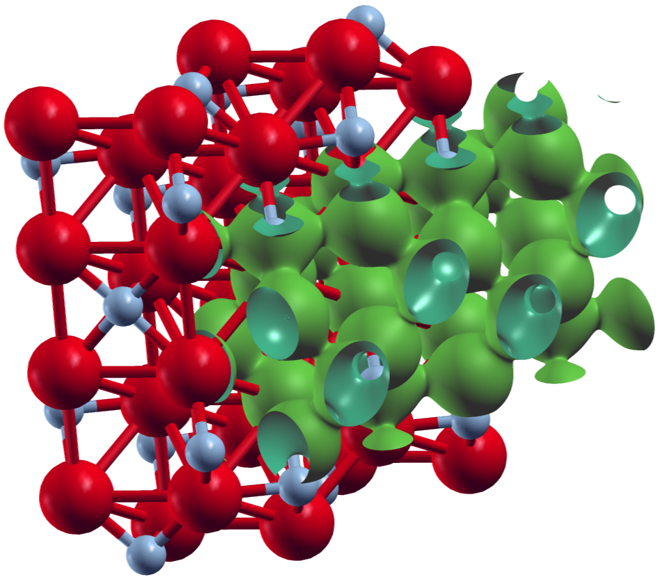
XCrySDen plot of an isosurface for the total charge density for $\text{Fe}_2 \text{N}$.

The second plot shows an isosurface indicating a vanishing magnetization density and a color-coded visualization of the magnetization density on a plane, both on top of the underlying structure.

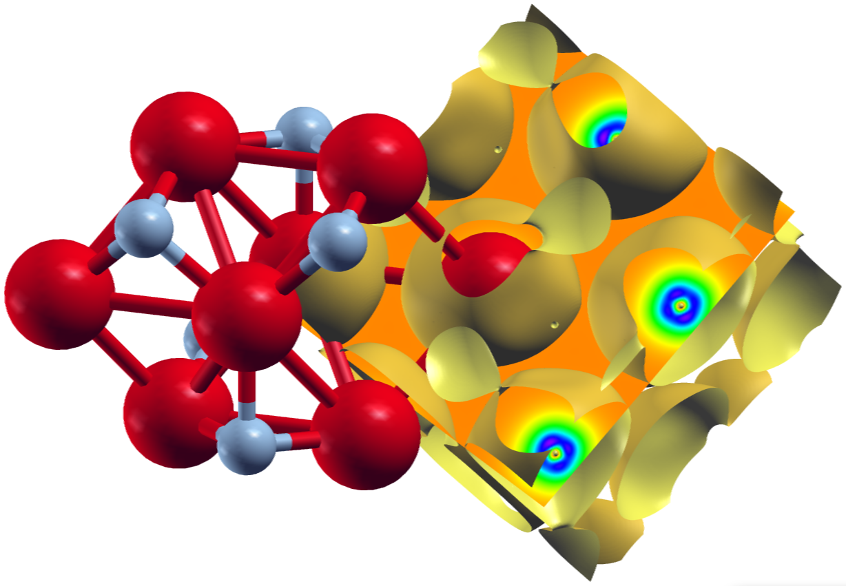
XCrySDen plot of the magnetization density for collinear ferromagnetic $\text{Fe}_2 \text{N}$.

The following input was used:

 1,xsf=T
 &PLOT twodim=f,cartesian=f
   vec1(1)=1.0 vec1(2)=0.0 vec1(3)=0.0 
   vec2(1)=0.0 vec2(2)=1.0 vec2(3)=0.0 
   vec3(1)=0.0 vec3(2)=0.0 vec3(3)=1.0 
   grid(1)=110 grid(2)=138 grid(3)=121 
   zero(1)=0.5 zero(2)=0.5 zero(3)=0.5 
   filename ='plot2' /

Note that the grid sizes in each direction differ. This has been done to achieve approximately cubic voxels in the datafile: The underlying unit cell is orthorombic. The offset defined by the zero in the plot_inp file is clearly visible in the plots above.

It is also possible to only plot the density contribution related to certain states which can be selected by different criteria. In Fleur this feature is called "charge density slicing". For this one first has to converge a self-consistent density and then prepare the plot by creating a charge density file that only contains the density due to the selected states. For the latter part of this procedure one has to set output/@slice to T and select the states in the output/chargeDensitySlicing tag.

It allows to specify the criteria by the following attributes:

• minEigenval: The minimal eigenvalue of the states to be selected. Investigate the eigenvalue in the out.xml file to select this value.
• maxEigenval: The maximal eigenvalue of the states to be selected. Investigate the eigenvalue in the out.xml file to select this value.
• pallst: Mnemonic for "plot all states", setting this boolean switch to T will also include the unoccupied states into the plot.
• nnne: This is used to specify a certain eigenstate index. If it is set to 0 the criterion is not applied.
• numkpt: This is used to specify a certain $\vec{k}$ point to be considered. If it is set to 0 the criterion is not applied.

Performing a Fleur calculation with such a parametrization will produce the desired charge density file cdn_slice.hdf or cdn_slice if Fleur is used without HDF5 support. Once this file is available one additionally sets output/plotting/@iplot to 2 and procedes with the plotting as before. The correct charge density file for the plotting will be chosen as long as output/@slice="T".

To illustrate this feature the following plot shows the density due to the defect states of an A-nitrogen center defect in the diamond bandgap at the $\Gamma$ point. A $4 \times 4 \times 4$ supercell was chosen for this calculation and the two nitrogen atoms are located on two opposing corners of the supercell. The plot visualizes an isosurface for some value of the density and an isolines-enhanced color-coding of the density on a plane on one side of the unit cell. Note that the color-plane is not parallel to the nitrogen bond.

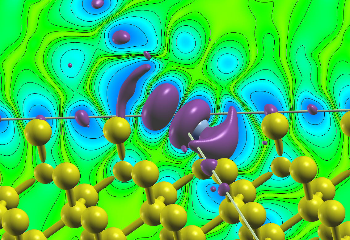
Density due to defect states of an A-nitrogen center defect in diamond.