
Parameter convergence
To obtain high-quality DFT calculations, their parametrization carefully has to be converged. In this section the dependence of Fleur calculations on the most-relevant parameters is discussed. Note that the convergence studies focus on the total energy. This may not be the quantity of relevance for the calculations a user has in mind. Due to fortunate error cancellations total energy differences converge much faster than total energies themselves. Thus, even if the default parametrization mentioned in the following discussions may seem to lead to underconverged results, for most quantities this is not of much relevance. However, it implies that the user has to ensure that the calculations he wants to compare feature analogous parametrizations. Otherwise differences may be dominated by unintended parameter changes.
Note that there is no optimal parameter set that works for all materials. The demands on the parameters depend on the actual physics in the material and are therefore material-dependent.
convergence
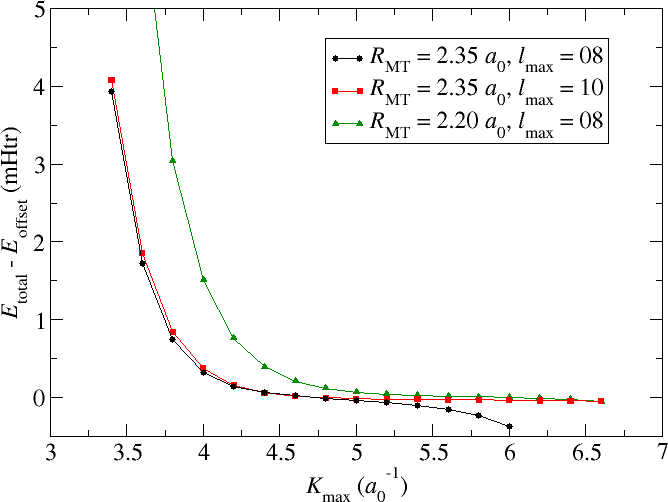
The example discussed in this section is an fcc Cu Crystal with a lattice constant of . The default parametrization generated by the input generator involved a MT radius of , a reciprocal plane wave cutoff for the LAPW basis of , and and angular momentum cutoff of . For such a setup the black curve in the following figure shows the dependence of the calculated total energy on an increasing cutoff. Note that and have manually been set to large enough values for all calculations. All energy values are provided relative to an arbitrary energy cutoff .
convergence for Cu
It can be seen that increasing the cutoff to values up to about leads to less and less changes in the total energy. Considering the fine energy scale one can assume that the total energy is converged for almost relevant applications. However, beyond the total energy shows an accelerating trend to ever lower values. Results for are not provided since the respective calculations crash.
What is observed here is the property of the LAPW basis to be nearly linearly dependent. Plane waves over the whole unit cell form, of course, an orthogonal basis set. But in the LAPW basis the plane waves only cover the interstitla region and in the MT spheres they are replaced up to some by numerical radial functions. Beyond the cutoff there is no replacement for the plane waves in the MT sphere. Considering the Rayleigh expansion of plane waves into spherical Harmonics on a sphere it is obvious that for larger cutoffs larger components become more and more important. Neglecting them in FLAPW yields the convergence behavior discussed above.
Fortunately there are obvious approaches to overcome such problems. One could either increase the cutoff as is shown by the red curve in the figure or reduce the MT radius as it has been done for the green curve.
Increasing the helps directly. The total energy becomes stable up to values of far beyond . However, since the numerical radial function is not the same as a spherical Bessel function that would actually perfectly replace the plane wave in the MT sphere, this approach might not always help. If it doesn't help one can still reduce the MT sphere radius. The respective curve also shows an increased stability up to very large values. But it is also obvious that a reduction of the MT radius implies the requirement to use larger parameters to obtain converged results. The product may actually be seen as a better convergence measure than alone.
Note that calculations performed with different MT radii might not yield the same results, even if they are carefully converged with respect to all other parameters. This is because of the relativistic treatment in the MT spheres which is not performed in the interstitial region. Also core electron states reaching out of the MT sphere may lead to a dependence of results on the MT sphere radius. Finally some output quantities are only evaluated in the spheres.
In the evaluation of the balance between these parameters one should also keep in mind that the number of LAPW basis functions is proportional to and the runtime of an SCF iteration is proportional to . This implies that the runtime is actually proportional to . For complex unit cells it is therefore advisable to choose a setup featuring already good convergence for small parameters.
and convergence
In contrast to increasing increasing is not problematic and will only yield more precise total energies. No calculation crashes or convergence problems due to too high parameters are known. However, the user should be aware that the requirements depend on the chosen parameter. A common way to choose is by using the rule of thumb
Increasing is also not problematic and will only yield more precise total energies. The difference to is that the requirements on are related to the potential in the respective MT sphere, while the requirements are due to the need to evaluate the kinetic energy of the Kohn-Sham orbitals with high precision and to avoid a linear dependence of the LAPW basis. This allows to choose smaller than . Typically they are chosen according to the rule
Both, and have to be systematically converged for every material under investigation. For most demands the default parameters from the input file generator are already good choices. Note that increasing these parameters is computationally expensive.
The linearization error
Within the MT spheres the LAPW basis features a linearized representation of the Kohn-Sham orbitals around the energy parameters defined in the input file. Of course, this implies that for energies different from the energy parameters there exists a linearization error. It depends quadratically on the energy difference between the energy parameters and the Kohn-Sham states.
For many structures the linearization error for the representation of the valence states is tiny and neglectable, but there are also setups, calculations, and quantities for which care has to be taken to overcome the linearization error and obtain high-quality results. Different strategies exist to eliminate the error. One approach is to shrink the MT sphere in which the error occurs. Another approach is to extend the basis in the respective MT sphere by local orbitals tailored to reduce the error.
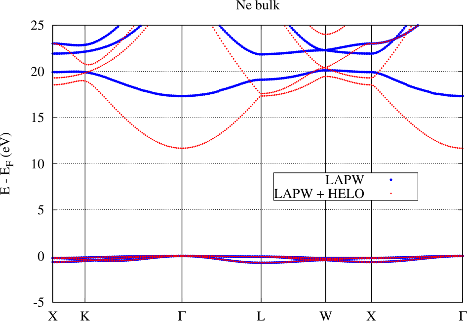
The following figure shows the band structure for an fcc Ne crystal obtained with the conventional LAPW basis and with an LAPW basis extended by local orbitals for higher energies in the range of the unoccupied bands (HELOs). The basic setup for these calculations involve the determination of energy parameters for the , , , and states and a MT radius of . For the HELO extended calculation a set of HELO type local orbitals for the , , , and states were added.
Linearization error for the Ne band structure.
It is directly visible that on the energy scale measurable in the plot the representation of the valence states by the conventional LAPW basis is already excellent: The bands calculated with the two setups lie on top of each other. But the LAPW basis functions are only constructed for the valence states. For the unoccupied bands in this example the representation is bad. Adding local orbitals to the basis overcomes this problem and a precise DFT bandgap can be extracted from the figure. Note, however, that Ne belongs to the most extreme examples for the effect of the linearization error on the predicted bandgap. To overcome the error it is also possible to strongly reduce the MT sphere radius, but this is computationally more expensive.
The demonstration of the effect of the linearization error on the unoccupied states may seem to have limited relevance, but certain calculations also rely on precise representations of these states. For example, GW calculations on top of DFT calculations require unoccupied states up to very high energies above the Fermi level as part of their input. For such calculations it may even be required to add multiple sets of HELOs to cover the whole energy range of relevance. For an analysis of the relevance of the linearization error on GW calculations see C. Friedrich et al., Band convergence and linearization error correction of all-electron GW calculations: The extreme case of zinc oxide, Phys. Rev. B 83, 081101(R) (2011).
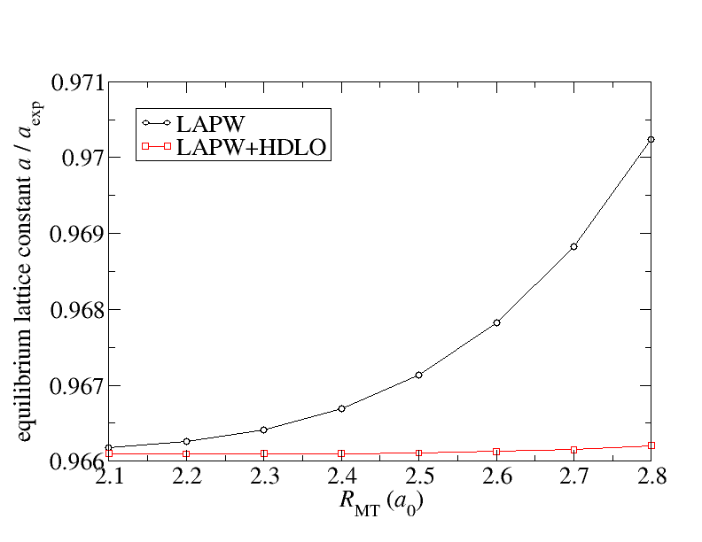
There are also cases for which the linearization error for the representation of the valence states is relevant. The consequence of this error may be a dependence of calculated quantities on the MT radius. The figure below sketches such an example. It displays the dependence of the calculated equilibrium lattice constant of KCl on the MT radius. The MT radii for both atom species were chosen to be identical.
MT radius dependence due to the linearization error for the KCl lattice constant.
The figure compares for this dependence the behavior for the conventional LAPW basis with that of an LAPW basis extended by a set of local orbitals (, , , states) constructed with the second energy derivative of the solution to the radial Schrödinger equation (HDLOs). It can be seen that the extended basis yields results that are stable against variations of the MT radius. This is the wanted behavior. Note that the lattice constant of KCl is especially sensitive to the linearization error due to the large MT spheres and its small bulk modulus. A more detailed analysis of the linearization error is performed in G. Michalicek et al., Elimination of the linearization error and improved basis-set convergence within the FLAPW method, CPC 184, 2670 (2013).
-point set convergence
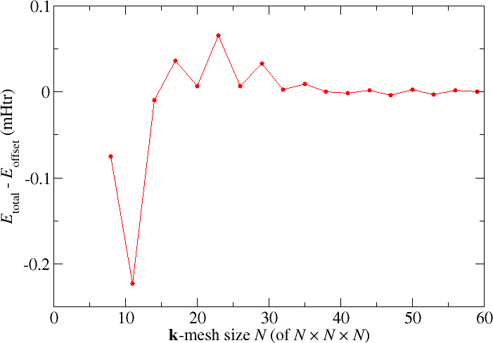
An aspect of the parametrization that is not limited to the FLAPW method is the choice of the -point set used to sample the Brillouin zone in the construction of the charge density. For the Cu example discussed above the Fleur input generator yields an -point mesh. The following figure shows how the results for the total energy change when finer -point meshes are selected
-point mesh convergence for Cu.
For this example the changes in the total energy are very small and for most purposes the default -point set is sufficient. For other unit cells and for certain target quantities this may be different and the -point mesh has to be chosen much finer. But even here it is important to choose analogous -point sets if different structures have to be compared, i.e., the -point density should be as similar as possible.
The plot also demonstrates an even-odd behavior: The convergence behavior differs between even and odd -mesh sizes . Such a behavior can also be observed in some other systems. It is related to the presence or absence of certain points in the set.
In general the demands on the -point set depend on the complexity of the electronic structure in the vicinity of the Fermi energy and the sensitivity of the investigated quantity on the details of the electronic structure in this energy range. This implies that for insulators rather coarse meshes are sufficient and for metals finer meshes are needed. Also the required mesh size is reciprocal to the unit cell size: The -point density should be chosen to be the same for primitive unit cells and for supercells.
numbands convergence for spin-orbit coupling in 2nd variation
When performing calculations involving the inclusion of spin-orit coupling (SOC) in second variation the number of bands to be taken into
account for the second variation step (numbands) also is a convergence parameter that has to be considered. In the following
figure the respective total energy convergence for such calculations on elemental bulk Pb is shown. The default number of bands taken
into account for this system is 24. Increasing the parameter yields the expected behavior, i.e., one obtains lower and lower total energies
until some minimal value is reached.
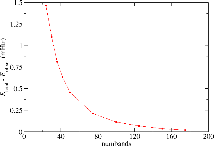
numbands convergence for SOC calculations on Pb.
Note that the convergence observed in the second variation step also relies on the LAPW basis. A change in the LAPW basis may lead to a behavior, e.g., one needs more bands but also reaches lower total energies. This is especially relevant since the radial functions in the MT spheres are not constructed for the description of spin-orbit coupling and it is hard to systematically converge the MT basis to obtain a high-quality representation for this purpose. The results of second variation SOC calculations therefore are approximative, though the approximation is good and allows quantitative predictions for many quantities.