1. Spin spirals

Magnetic materials can feature spin-spiral ground states. In such structures the magnetic moment at some atom is rotated by a fixed angle when going to the next atom of this kind in a certain direction defined by the wavevector of the spin spiral $\vec{q}$. The periodicity of this spin spiral might not coincide with the periodictity of the chemical unit cell or some supercell. Nevertheless we can describe such systems with arbitrary periodictity by employing the generalized Bloch theorem.

1.1 Spin-spiral ground state in fcc Fe

In its ground state Fe crystallizes in a bcc structure, but it is also possible to synthesizes Fe in an fcc structure, e.g., fcc Fe clusters may form by fast annealing of Fe in a Cu matrix.

It is known that the magnetic ground state of such an fcc Fe structure is a spin spiral. In this exercise we will determine this magnetic structure by minimizing the total energy with respect to the $\vec{q}$-vector (wavevector) of the spin spiral.

Set up an fcc Fe input with the Cu lattice constant of $6.82~a_0$ and add the following line to the end of the inpgen input:

&qss 0.5 0.5 0.0 /

With this inpgen will generate a Fleur input file with the correct symmetries for the provided $\vec{q}$-vector qss. Generate a Fleur input file with the inpgen option -noco to also write out the parametrization for noncollinear calculations.

The provided $\vec{q}$-vector will rotate the magnetic moment in the MT sphere with respect to the atom position around the z axis. Since by default the magnetic moment points in the z direction this will not have any effect. To actually observe an effect we now tilt the magnetic moment into the xy-plane. This is done by changing the $\beta$ angle in the nocoParams tag of the Fe atom to $\pi/2.0$.

With such a setup we have defined a spin spiral in the xy-plane. The rotation of the magnetic moment for an atom at $\vec{\tau} = (\tau_x,\tau_y,\tau_z)$ (in internal coordinates) is $2\pi\langle \vec{q} \vert \vec{\tau} \rangle$. The chosen $\vec{q}$-vector thus rotates the magnetic moment from unit cell to unit cell by $\pi$. We therefore describe an antiferromagnetic fcc Fe crystal with this setup.

We observe that the $\vec{q}$-vector in calculationSetup/nocoParams/qss was not taken over from the inpgen input (due to a bug). We change it such that the first two coordinates are set to 0.5 and the last one stays 0.0. We want to perform several calculations with different $\vec{q}$-vectors.

We also observe that by default the switches calculationSetup/magnetism/@l_noco and calculationSetup/nocoParams/@l_ss are set to true. This is because of the definition of a $\vec{q}$-vector in the inpgen input. This means that we already activated noncollinear calculations with a rotation of the orientation of the magnetic moment in the Fe MT sphere from unit cell to unit cell.

For the following calculation series we will adapt a few parameters to reduce the runtime and obtain a slightly better convergence behavior. Set calculationSetup/scfLoop/@itmax to 90, calculationSetup/scfLoop@minDistance to 0.0005, calculationSetup/scfLoop/@maxIterBroyd to 15, and use

<kPointMesh nx="7" ny="7" nz="7" gamma="F"/>

for the definition of the $\vec{k}$-point set. Please also execute

export OMP_NUM_THREADS=4

on your computer to enable the usage of 4 OpenMP threads.

Note: Some calculations will feature an incompletely convergence with respect to the charge density. But the total energies should be stable.

Perform the calculations for x-, y-coordinates (qXYCoord) of the $\vec{q}$-vector ranging from $0.0~a_0^{-1}$ to $0.5~a_0^{-1}$ in steps of $0.05~a_0^{-1}$ and generate a data file with two columns: qXYCoord vs. total energy. Plot the file. Which $\vec{q}$-vector minimizes the total energy? Your results should be similar to the following plot.

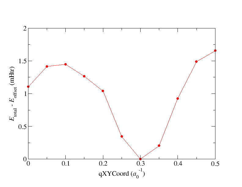
Spin-spiral dispersion relation for fcc Fe.

2. Exercises

2.1 Spin-spiral ground state in fcc Fe with the magnetic force theorem

Similarly to the magnetocrystalline anisotropy spin-spiral dispersions can also be obtained with the magnetic force theorem. Do this for the system sketched in task 1.1. As a starting point you need a converged calculation for some q point (best in a separate directory). Once you have this change the number of iterations to be performed to $1$ and add a block for the force theorem as last entry in the fleurInput tags. This block has the form

<forceTheorem>
   <spinSpiralDispersion>
      <q> 0.00 0.00 0.0 </q> <!-- This has to be the same q vector you use for obtaining the self-consistent solution. -->
      <q> 0.05 0.05 0.0 </q>
      <!-- Further q vectors can be specified here. -->
   </spinSpiralDispersion>
</forceTheorem>

Perform two calculations, one with an initial q vectors $(0.0, 0.0, 0.0)$ and one with an initial q vector $(0.3, 0.3, 0.0)$. Compare the dispersion relations obtained from the eigenvalue sums with the one obtained from the total energies of the exact calculation in 1.1.

Note: The results will be rather bad. Maybe due to suboptimal parameter convergence, maybe due to the choice of the initial q vector, maybe due to a variation in the physics over the different q vectors bringing the force theorem to its limits.

Results to be delivered: One plot with the three spin-spiral dispersion relations.