Description of spin spirals

Spin spirals are periodic magnetic structures that can be described by a vector field. For a rotation axis along the z direction their magnetization $\vec{M}$ is given by:

$\begin{equation} \renewcommand{\vec}[1]{\mathbf{#1}} \mathbf M_{n,\mu} = M \left(\begin{matrix} \cos(\vec{q} \cdot (\vec{R}_{n} + \vec{\tau}_{\mu}) + \alpha_{\mu}) \sin(\beta_{\mu}) \\ \sin(\vec{q} \cdot (\vec{R}_{n} + \vec{\tau}_{\mu}) + \alpha_{\mu}) \sin(\beta_{\mu}) \\ \cos(\beta_{\mu}) \end{matrix}\right) \end{equation}$

where $\vec{R}_{n}$ is the lattice vector pointing from the origin to unit cell $n$ , $\vec{\tau}_{\mu}$ is the position of atom $\mu$ in the unit cell, $\vec{q}$ is the so called spin-spiral vector, $\beta_{\mu}$ is the cone angle between the magnetic moment of atom $\mu$ and the rotation axis, and $\alpha_{\mu}$ is an atom-dependent phase shift.

In general, the period length $\lambda = \frac{2\pi}{q}$ can be many times larger than a lattice period. Hence it is not feasible to simulate a spin spiral directly because one would need to use extremely large supercells. However, in the absence of spin-orbit coupling, the generalised Bloch theorem allows to overcome this problem. The theorem states that a wave function of a system featuring a spin spiral can be represented as:

$\begin{equation} \psi_{\mathbf k} (\mathbf r) = \left( \begin{matrix} e^{i(\mathbf k - \mathbf q/2) \cdot \mathbf r} u^{\uparrow}_{\mathbf k} (\mathbf r) \\ e^{i(\mathbf k + \mathbf q/2) \cdot \mathbf r} u^{\downarrow}_{\mathbf k} (\mathbf r) \end{matrix} \right) \end{equation}$

In Fleur the description of spin spirals is part of the code treating noncollinear magnetism [1]. This implies that one should invoke the input generator with the -noco or -explicit command line switches to obtain templates for the parametrization of calculations on noncollinear magnetism. Next, the treatment of noncollinear magnetism has to be activated by setting calculationSetup/magnetism/@l_noco to T. The angles $\alpha_{\mu}$ and $\beta_{\mu}$ are set in the atomGroups/atomGroup/nocoParams/@alpha and atomGroups/atomGroup/nocoParams/@beta attributes. To finally switch on the calculation of a spin spiral by employing the generalized Bloch theorem also calculationSetup/magnetism/@l_ss has to be set to T. The following example demonstrates such a setting.

<magnetism jspins="2" l_noco="T" l_ss="T">
   <qss>0.25 0.25 0.0</qss>
</nocoParams>

The $\vec{q}$ vector is set in the qss tag enclosed by calculationSetup/magnetism and measured in reciprocal lattice vectors.

To ensure that the symmetry operations found for the unit cell are not incompatible to the $\vec{q}$ vector, the inpgen input should be extended by a line specifying the $\vec{q}$ vector. For the here-considered $\vec{q}$ this line is &qss 0.25 0.25 0.0 /.

Under the assumption that the setup in the example above belongs to an fcc unit cell with the Bravais matrix

$\begin{equation} A = \frac{a}{2} \cdot \left( \begin{matrix} 0.0 & 1.0 & 1.0 \\ 1.0 & 0.0 & 1.0 \\ 1.0 & 1.0 & 0.0 \end{matrix} \right) \end{equation}$

the reciprocal unit cell would be defined by the matrix

$\begin{equation} B = \frac{2\pi}{a} \cdot \left( \begin{matrix} -1.0 & 1.0 & 1.0 \\ 1.0 & -1.0 & 1.0 \\ 1.0 & 1.0 & -1.0 \end{matrix} \right) \end{equation}$

which defines a bcc-like structure. This implies that the defined $\vec{q}=(0.25,0.25,0.0)$ would point in z direction for this example.

The magnetic moment of an atom at position $\vec{\tau}$ (internal coordinates) is rotated by $2 \pi (\vec{q} \cdot \vec{\tau})$ . For the given example and $\beta=\pi/2$ this implies that an increase of the $\vec{q}$ vector to $\vec{q}=(0.5,0.5,0.0)$ would yield a layered structure with an antiferromagnetic alignment of the magnetization directions along z.

The following figure demonstrates different spin spirals that may be obtained with respective parametrizations in the Fleur input file.

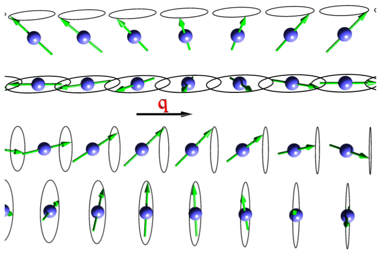
Four examples of spin spirals with spin-rotation axis perpendicular (upper two) and parallel (lower two) to the spin-spiral vetor $\vec{q}$ . For each case two spirals with angles of $\beta=\pi/4$ and $\beta=\pi/2$ between the magnetic moment and the rotation axes are shown. Figure taken from: Philip Kurz, Non-Collinear Magnetism at Surfaces and in Ultrathin Films (PhD Thesis, RWTH Aachen).

In the absence of spin-orbit coupling (SOC) the direction of the rotation axis is energetically irrelevant, therefore the first and third spin-spiral in the figure are equivalent (the same applies to the second and fourth one). For convenience, if no SOC is considered the rotation axis is always set to point in z-direction. I.e., if the magnetization of an atom points along z, it will not rotate. If it points in x-direction ( $\beta=\pi/2$ ), it describes a flat spiral (second example of the figure).

The description of spin spirals in this way is incompatible to the inclusion of spin-orbit coupling in the calculation. If spin spirals have to be calculated under consideration of SOC this can be done by employing the magnetic force theorem.

Like all other calculations on noncollinear magnetism, spin-spiral calculations are incompatible to the exact treatment of the core-electron tails reaching out of the MT spheres. Thus calculationSetup/coreElectrons/@ctail has to be set to F

Since the number of basis functions changes (slightly) with $\mathbf q$ , for consistent output quantities it is important that the basis cutoff ( $K_\text{max}$ ) is not too small, typically increased by 0.5 - 1.0 as compared to normal non-collinear calculations. Also, a dense $\mathbf k$ -grid is recommended when sampling $\mathbf q$ space, usually twice as dense as the $\mathbf q$ -grid works best [3].

Further reading

Keys	Action
`?`	Open this help
`n`	Next page
`p`	Previous page
`s`	Search