
Plotting densities and potentials
The FLEUR code offers several options of plotting the densities and potentials. The feature is MPI and OMP parallelized and can be applied to systems of reasonable size to gain insight about their electronic structure. However, care needs to be taken when choosing the number of MPI processes. It should be a divisor of the number of grid points in z-direction.
The corresponding switches can be found in the output section of the Fleur
input file under
<plotting iplot="0" polar="F" format='1'>
</plotting>
With the above information, no plot will be created yet. To do so, first run a normal
self-consistency calculation and then modify the inp.xml by setting iplot to a
particular integer. Another iteration will be executed during which several
quantities can be plotted out. The new density from this iteration is not written
into the density file. The plottable quantities are:
- The input density as generated by the density file from the self-consistent run [id=1, name=denIn].
- The total potential calculated from the input density that goes into the Kohn- Sham-Equations [id=2, name=vTot].
- The Coulomb potential calculated from the input density [id=3, name=vCoul].
- The exchange-correlation potential [id=4, name=vXc].
- The output density calculated before it is mixed with the input for the next iteration [id=5, name=denOutWithCore].
- The mixed density calculated for the next iteration [id=6, name=denOutMixWithCore].
To control the options via a single integer switch, iplot is calculated by
binary addition from the plot ids given above. For example, if you want to plot the
input density and the resulting potential, then iplot=2^1+2^2=2+4=6. Optionally,
iplot=1 or any odd number will plot all options coded into FLEUR. The polar switch will, when set to
true, generate additional plots in the non-collinear case, id est for example the
magnetization density components in x-, y- and z-direction will be supplemented
by the absolute values |m| and the angles and , giving the polar
representation. format can either be set to 1 or 2. 1 gives .xsf files to be used
with XCrySDen and 2 will print out all available information and coordinates as a
tabloid.
To generate plots, another tag needs to be added into the inp.mxl file in the plotting section:
<plot cartesian="F" TwoD="T" grid="30 30 30" vec1="1.0 0.0 0.0" vec2="0.0 1.0 0.0" vec3="0.0 0.0 1.0" zero="0.0 0.0 0.0" file='plot' onlyMT='F' typeMT='0' vecField='F'/>
There can be multiple tags of this form to make plots with different characteristics.
If at least one tag is put in, a plot will be made, otherwise setting iplot
to a non-zero integer will have no effect. The various plotting options can now be
specified. Note, that not all particular switches need to be given, as defaults exist.
The examplary tag contains the default options coded into FLEUR. The tag contains the
following options:
- cartesian: Are the following options given in internal or cartesian (Bohr radii) units?
- TwoD: Determines whether a 2-dimensional or 3-dimensional density plot is created.
- grid: Number of grid points in each direction.
- vec: Bravais matrix of the system in question.
- zero: Origin shift of the plot.
- file: Name of the plot. This will be [part of] the filename for non-xsf or vector plots and an identifying tag in xsf-datagrids otherwise.
- onlyMT: When set to true, all gridpoints not in the Muffin Tins will have zero density to better visualize the atomic densities.
- typeMT: More specific than the last switch, this one will set everything to zero except for a single type of atoms specified by an integer n.
Note, that cartesian units within FLEUR are done in units if the Bohr radius , while XCrySDen operates in Angstrom. All output files will have their coordinates written in the latter.
To better understand which files are written, here are some examples for the case
of a single 3D plot with iplot='2', polar='F' and format='1' in the
plotting tag and TwoD='F' for the different levels of magnetism:
- non-spinpolarized:
denIn.xsfwith a singleDATAGRIDcalled "plot". - collinear:
denIn_f.xsfanddenIn_g.xsfeach with a singleDATAGRIDcalled "plot". These are the total and magnetization density. - non-collinear:
denIn_f.xsf,denIn_A1.xsf,denIn_A2.xsf,denIn_A3.xsfeach with a singleDATAGRIDcalled "plot". These are the total density and the three components of the magnetization density. - non-collinear with
polar=T:denIn_f.xsf,denIn_A1.xsf,denIn_A2.xsf,denIn_A3.xsf,denInAabs.xsf,denInAtheta.xsf,denInAphi.xsfeach with a singleDATAGRIDcalled "plot". These are the total density, the three components of the magnetization density and their polar representation. - non-collinear with
vecField=T:denIn_f.xsf,denIn_A1.xsf,denIn_A2.xsf,denIn_A3.xsfanddenIn_A_vec_plot.xsf
The descriptors in the filenames refer to the representations as scalar fields and or the components of a vector field . For the potential, these quantities correspond to the effective scalar potential and the additional exchange-correlation magnetic field in the spin-polarized case.
Using the representations of forces in XCrySDen, plots of the vectorial quantities
can also be made. For this, set vecField=T in a non-collinear calculation (for
collinear spin-polarized calculations please use the above example and view the _f
and _g quantities). The vector for each grid point will be written into a new file
as an atom of type X at coordinates x, y, z, with the associated "Forces" Ax, Ay and
Az. In the file, manually set the first number under PRIMCOORD from n up to n
plus the total number of gridpoints specified. Dummy atoms will then be displayed
in the XCrySDen visualization and the vectors can be shown by going to Display
and checking Forces. In the Modify section, the representation of these vectors
can then be controlled. Note, that it is quite hard to neatly visualize the vectors,
as the length and thickness needs to be chosen appropriately and the atomic radius
of the dummies needs to be set very small. The visualization can easily become cluttered.
The following shows two plots created for a converged calculation on collinear ferromagnetic .
They were obtained in XCrySDen by reading in the denIn_f.xsf and denIn_g.xsf
to obtain the total density and magnetization density respectively.
The first plot shows an isosurface for a certain charge density value on top of the structure extended to two unit cells in y- and z-direction.
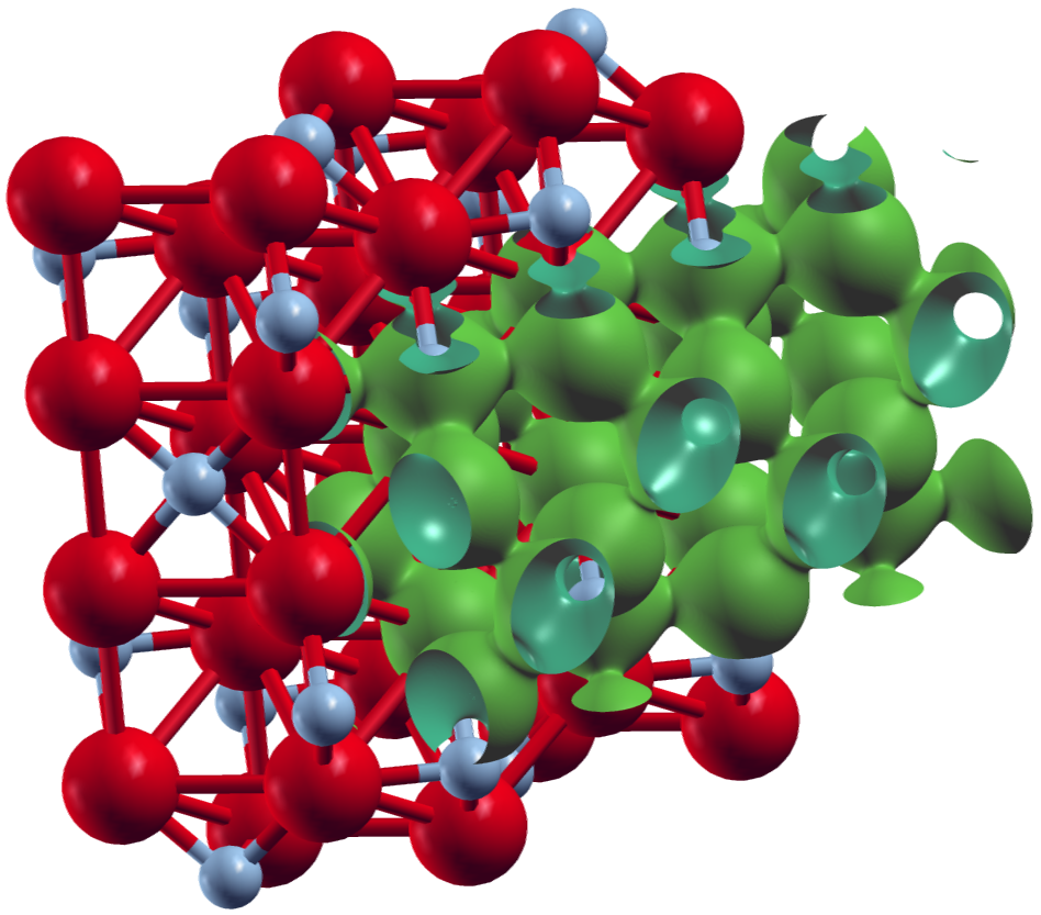
XCrySDen plot of an isosurface for the total charge density for .
The second plot shows an isosurface indicating a vanishing magnetization density and a color-coded visualization of the magnetization density on a plane, both on top of the underlying structure.
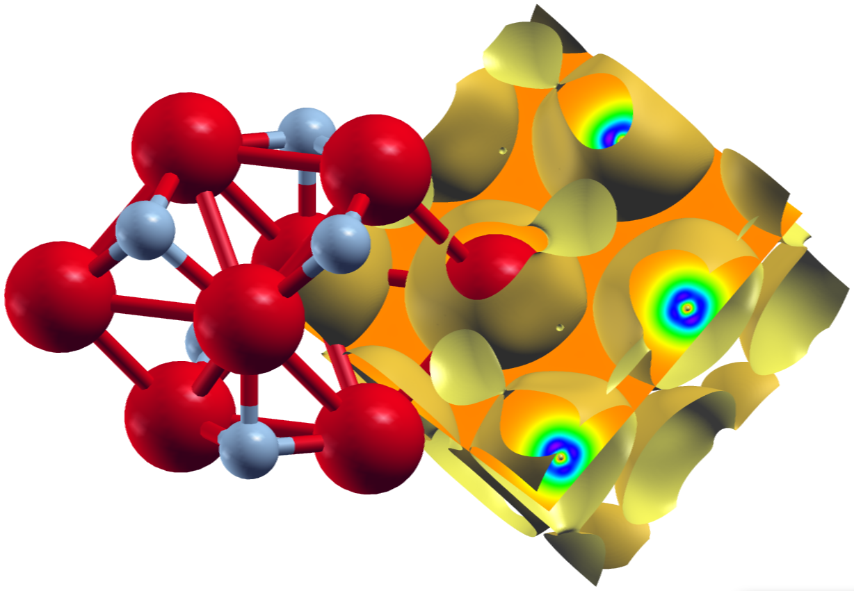
XCrySDen plot of the magnetization density for collinear ferromagnetic .
The following input was used:
<plotting iplot="2" polar="F" format='1'/>
   <plot cartesian="F" TwoD="F" grid="110 138 121" vec1="1.0 0.0 0.0" vec2="0.0 1.0 0.0" vec3="0.0 0.0 1.0" zero="0.5 0.5 0.5" file='plot2'/>
</plotting>
Note that the grid sizes in each direction differ. This has been done to achieve approximately cubic voxels in the datafile:
The underlying unit cell is orthorombic. The offset defined by the zero in the tag is clearly
visible in the plots above.
It is also possible to only plot the density contribution related to certain states which can be selected by different criteria.
In Fleur this feature is called "charge density slicing". For this one first has to converge a self-consistent density and
then prepare the plot by creating a charge density file that only contains the density due to the selected states. For the latter
part of this procedure one has to set output/@slice to T and select the states in the output/chargeDensitySlicing tag.
It allows to specify the criteria by the following attributes:
minEigenval: The minimal eigenvalue of the states to be selected. Investigate the eigenvalue in theout.xmlfile to select this value.maxEigenval: The maximal eigenvalue of the states to be selected. Investigate the eigenvalue in theout.xmlfile to select this value.pallst: Mnemonic for "plot all states", setting this boolean switch toTwill also include the unoccupied states into the plot.nnne: This is used to specify a certain eigenstate index. If it is set to0the criterion is not applied.numkpt: This is used to specify a certain point to be considered. If it is set to0the criterion is not applied.
Performing a Fleur calculation with such a parametrization will produce the desired charge density file cdn_slice.hdf or cdn_slice
if Fleur is used without HDF5 support. Once this file is available one additionally sets output/plotting/@iplot to 2 and procedes
with the plotting as before. The correct charge density file for the plotting will be chosen as long as output/@slice="T".
To illustrate this feature the following plot shows the density due to the defect states of an A-nitrogen center defect in the diamond bandgap at the point. A supercell was chosen for this calculation and the two nitrogen atoms are located on two opposing corners of the supercell. The plot visualizes an isosurface for some value of the density and an isolines-enhanced color-coding of the density on a plane on one side of the unit cell. Note that the color-plane is not parallel to the nitrogen bond.
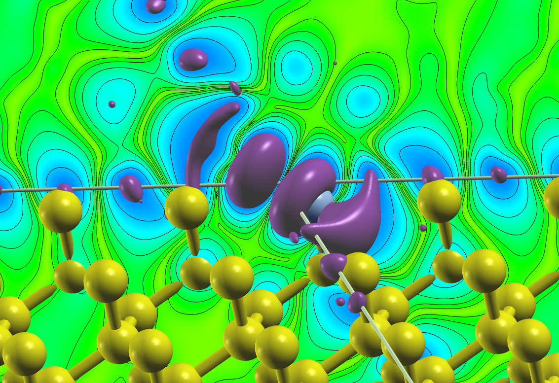
Density due to defect states of an A-nitrogen center defect in diamond.